______________________________
STRUCTURAL 3D MONITORING USING A NEW SINUSOIDAL FITTING
ADJUSTMENT
I. Detchev a,*, A. Habib b, D. Lichti a, M. El-Badry a
a Dept. of Geomatics Engineering & c Dept. of Civil Engineering, University of Calgary, 2500 University Dr NW, Calgary, Alberta, T2N 1N4 Canada - (i.detchev, ddlichti, melbadry)@ucalgary.ca
b
Lyles School of Civil Engineering, Purdue University, 550 Stadium Mall Drive, West Lafayette, Indiana, 47907-2051 USA - [email protected]
Commission V, WG V/1
KEY WORDS: close range photogrammetry, dynamic loading, precise 3D reconstruction, image and point cloud processing, model-based image fitting, vertical deflections, planimetric displacements
ABSTRACT:
Digital photogrammetric systems combined with image processing techniques have been used for structural monitoring purposes for more than a decade. For applications requiring sub-millimetre level precision, the use of off-the-shelf DSLR cameras is a suitable choice, especially when the low cost of the involved sensors is a priority. The disadvantage in the use of entry level DSLRs is that there is a trade-off between frame rate and burst rate – a high frame rate is either not available or it cannot be sustained long enough. This problem must be overcome when monitoring a structural element undergoing a dynamic test, where a range of loads are cycled through multiple times a second. In order to estimate deflections during such a scenario, this paper proposes a new least-squares adjustment for sinusoidal fitting. The new technique is capable of processing multiple back-to-back bursts of data within the same adjustment, which synthetically increases the de-facto temporal resolution of the system. The paper describes a beam deformation test done in a structures laboratory. The experimental results were assessed in terms of both their precision and accuracy. The new method increased the effective sampling frequency three-fold, which improved the standard deviations of the estimated parameters with up to two orders of magnitude. A residual RMSE as low as 30 µm was attained, and likewise the RMSE of the computed amplitudes between the photogrammetric system and the control laser transducers was as small as 34 µm.
1. INTRODUCTION
Infrastructure health monitoring is essential for both safety and serviceability. Routine inspections and maintenance operations are employed for already existing structures. The maximum load-carrying capacity for new structures is estimated and individual components are tested as part of the design process. A common check performed on a structural element is the measurement of deflections at particular locations of interest. This is necessary to verify that any occurring deformations are within the allowable limits (Brownjohn, 2007).
1.1 Traditional Infrastructure Monitoring Instrumentation
Deformation monitoring of structural elements has traditionally been implemented with strain gauges, optical fibre sensors and/or laser transducers. Some of these instruments achieve high precision and can collect data at a high frequency; however, there are multiple practical problems associated with their use. They are either contact instruments and require access to the monitored area, or they have a limited range, so the measurements must be carried out from a close distance. This imposes a risk of damage in the case of failure of the specimen being tested (Gordon and Lichti, 2007). It is not economically feasible or logistically practical to use dozens of instruments to have complete coverage (Maas and Hampel, 2006), so trained and experienced personnel must select specific points to be monitored. These instruments perform measurements in one dimension/direction only (Gordon and Lichti, 2007; Jiang et al., 2008; Maas and Hampel, 2006). No permanent visual record (Whiteman et al., 2002) is formed unless some basic notes are written with a marker directly on the specimen.
1.2 Optical Imaging Modalities for Infrastructure Monitoring
Overcoming the downsides or complementing the limitations of the traditional instrumentation can be accomplished by the use of optical imaging modalities. Remote sensing techniques such as terrestrial laser scanning (Gordon and Lichti, 2007; Park et al., 2007) and digital photogrammetry (Fraser and Riedel, 2000; Jáuregui et al., 2003; Mills et al., 2001) have been used for over a decade. Recently, range or 3D cameras have also been employed (Lichti et al., 2012). These techniques are capable of reconstructing entire 3D surfaces (Lichti et al., 2000) from a safe distance, which can be used for making precise deflection measurements. Also, a permanent visual record is established for every observed epoch (Jiang and Jáuregui, 2007).
The type(s) of sensor(s) employed during a data collection campaign should be decided on per-application basis depending on the size of the specimen monitored, the type of loading applied, and the budget of the project. The specimens could be concrete beams, T-shaped beam-column joints or truss girders with lengths of 3 m or more. The loading procedure could be static or dynamic. In static testing, the load applied to a specimen is progressively increased. As a result the tested specimen deflects typically at a slow rate (e.g., a millimetre every few minutes). In dynamic or fatigue testing, a range of loads is repeatedly cycled through at a rate appropriately simulating real-world operating conditions such as vehicle traffic on a bridge. Thus, the motion of the specimen resembles a sinusoidal curve, and its vertical deflection can range in the order of several millimetres every second or a few times every second. The cost of the sensors may vary from a few hundred dollars for a 2D digital camera or a gaming 3D camera to tens ISPRS Annals of the Photogrammetry, Remote Sensing and Spatial Information Sciences, Volume III-5, 2016
or hundreds of thousands of dollars for a commercial laser scanner.
For static scenes, where a constrained budget is not an issue, laser scanning performs more than satisfactory (Rönnholm et al., 2009). For kinematic objects, where precision at the sub-errors and in some cases synchronization between multiple sensors is not possible.
1.3 Advantages and Disadvantages of 2D Digital Cameras
This paper focuses on the use of low-cost off-the-shelf 2D digital cameras in order to precisely reconstruct entire surfaces of (a) kinematic object(s) in a structural laboratory setting. The most suitable 2D cameras for photogrammetric purposes are the digital single-lens reflex (DSLR) or the mirrorless types with the capability of interchanging lenses. This is because they normally have larger sensor sizes and the user is given full control over the drive mode, the exposure and the focus settings of the camera. Having a larger sensor size usually yields images with higher spatial resolution, which are also less prone to noise in low light conditions. Having control over the camera settings helps minimize any potential photo variations within a block, and given a rigorous geometrical calibration is performed, the camera can be treated as a metric one (Fraser, 1997; Habib and Morgan, 2003).
The disadvantage of employing DSLR cameras, especially the entry level ones, is that the operator faces a trade-off between frame rate and burst rate. Frame rate is the sampling frequency of the sensor, and can be used as a measure for its temporal resolution. Burst rate is the maximum number of consecutive files that a camera can output at a constant frame rate in continuous shooting mode. Due to limitations in its memory buffer and/or processor, a camera which produces large file size still images typically either does not have a high frame rate or its frame rate cannot be sustained long enough. In a multi-camera photogrammetric system this may lead to a breakdown in the synchronization between the cameras.
1.4 Research Objectives
The goal of this research initiative is to use a photogrammetric system consisting of multiple digital cameras for the purposes of monitoring specimens during dynamic loading tests. The images acquired with the system from every observation epoch would be post-processed as to reconstruct and track features describing the deflections or displacements of the structural element. Since the behaviour of the specimen can be modelled using a sinusoidal curve, a least-squares sinusoidal fitting adjustment can be applied on the data to estimate the motion parameters (Detchev et al., 2014a, 2013; Qi et al., 2014a, 2014b). In order to overcome the sampling issues of 2D off-the-shelf digital cameras, this paper proposes a least-squares adjustment, which enables the processing of multiple back-to-back bursts of data. The idea is that the use of multiple bursts would synthetically increase the de-facto frame rate or the sampling frequency of the system. This would allow for the reliable use of an otherwise slow system for the observation of structural elements being tested at high loading frequencies.
The rest of the paper first explains the methodology for 3D monitoring of structural elements, and in particular the newly proposed adjustment for sinusoidal fitting. The paper describes the system setup, an experiment on a concrete beam in a structures laboratory, and the conducted procedures for extracting the trackable features for the given specimen. Finally, the paper discusses the results from the conducted dynamic loading test in terms of both the precision and accuracy of the estimated parameters.
2. METHODOLOGY FOR 3D MONITORING OF STRUCTURAL ELEMENTS
The proposed methodology for 3D monitoring of structural elements consists of three parts: 1) procedures for quality assurance; 2) image and point cloud processing for the reconstruction and extraction of trackable features in each observed epoch; and 3) running a geometrical fitting adjustment of the extracted features in order to estimate preferably the 3D motion of the monitored specimen.
2.1 Quality Assurance Procedures
In order to achieve precise 3D photogrammetric reconstruction, it is essential to have a valid system calibration done prior to the field campaign or in-situ. In addition, good quality images must be collected during the actual data acquisition campaign.
2.1.1 System calibration: A photogrammetric multi-camera system calibration consists of two parts. One part is the geometrical calibration or estimating the interior orientation parameters (IOPs) of each camera. The other part is the estimation of the position and orientation or the exterior orientation parameters (EOPs) of each camera with respect to an object space reference frame or a reference camera. Ideally, the two parts of the system calibration should be done in a single bundle adjustment. Once the cameras are set up in a particular laboratory, calibration data should be collected in-situ prior to the commencement of the actual test. Convergent camera station geometry (including rolled images) must be ensured for all the involved cameras in addition to guaranteeing that there is sufficient overlap between at least each neighbouring pair of cameras. This can be achieved by translating and rotating a test field with signalized targets in front of the system (Detchev et al., 2014b).
2.1.2 Data collection considerations: In the case of a specimen with large homogeneous surfaces, signalized targets or plates with distinct geometrical shape can be stuck to the object of interest, so any changes in their coordinates can be photographed during the data acquisition. The field of view of the cameras should overlap so each feature or surface of interest is seen by a minimum of two, but ideally three or four cameras. The cameras must be set to manual driving mode and configured so that the images are correctly exposed and there is no motion blur. The cameras must also be synchronized so all the images from a particular epoch are taken at the same time and share the same shutter speed/integration time.
2.2 Image and Point Cloud Processing
Any trackable features or surfaces on the visible portions of the monitored specimen must be reconstructed and identified in every observed epoch. Multiple light ray intersection is used for the 3D reconstruction in this work. The matching of conjugate pixels is performed through a combination of area- and feature-ISPRS Annals of the Photogrammetry, Remote Sensing and Spatial Information Sciences, Volume III-5, 2016
based matching, where the corner detector of choice is the Harris operator (Harris and Stephens, 1988). The resulting point clouds must then be reduced to a list of 3D coordinates, where each set of coordinates represents the position of a tracked feature at a particular observation epoch.
2.3 Sinusoidal Fitting for Specimen Motion Estimation
Of interest in this research study is estimating the vertical, and if possible the planimetric, motion amplitude of each tracked feature for a series of observed epochs. As mentioned earlier, during a fatigue/dynamic loading experiment a specimen is repeatedly subjected to a range of loads; the vertical deflection, and if present the horizontal displacement, of each tracked feature exhibits a cyclic motion. This cyclic motion can be modelled as the following sinusoidal curve:
� = ∙ sin � ∙ � ∙ � + � + (1)
where is the observed height or depth of the signal at time �, and the unknown parameters are the amplitude ( ), the frequency (�), the phase (�), and the mean value ( ) of the signal (see Figure 1 for a visual example). The same equation can be used for the observed planimetric coordinates and . Even though the primary concern is the recovery of the amplitude, the other three parameters must be estimated as nuisance parameters. Since the sinusoidal curve model is non-linear, approximate values for the unknown parameters have to be provided, and the final values for these parameters are computed in an iterative manner. One way of deriving an approximate value for the frequency is through a Fourier transformation of the signal (Brigham, 1988). This will only work if the sampling frequency of the system is at least twice the frequency of the loading signal, i.e., it abides by the Nyquist theorem. The approximate values for the other parameters can be derived using the linear fundamental harmonic equation:
� = ∙ sin � ∙ � + ∙ cos � ∙ � + (2)
where � = � ∙ �. The parameters and can be used to retrieve the amplitude and phase according to (3) and (4):
= √ + (3)
� = tan− ( ) (4)
Figure 1 shows an example of a well-sampled signal, and gives a visual description of the four sought after sinusoidal fitting parameters. In this scenario, a reliable adjustment can be run for each tracked feature separately. The columns of the design matrix for each separate adjustment are shown in Figure 2.
Figure 1. Example of a 1 Hz signal sampled at 20 Hz
� �
Figure 2. The unknowns for a sinusoidal fitting adjustment where each available feature is dealt with separately While this traditional approach for sinusoidal fitting has been shown to work (Detchev et al., 2014a, 2013; Qi et al., 2014a, 2014b), it does not always produce reliable results for camera systems with low frame or burst rates. A low frame rate may yield data with sparse sampling of the signal, while a low burst rate may cover a limited number of cycles or not even a single complete cycle. Moreover, if the sampling frequency of the system does not abide by the Nyquist theorem, the adjustment may converge to an aliased frequency, and thus yield incorrect amplitude. The following two modifications to the sinusoidal fitting adjustment proposed next will address these issues. 2.3.1 Combine all features within a burst: One way of strengthening the sinusoidal fitting solution is to combine all tracked features within a burst in the same adjustment:
� = ∙ sin � ∙ � ∙ � + � + (5)
where � indicates the feature number. While the features will have different amplitudes and mean signal values, the assumption here is that there is only one load source, and all the features belong to a single specimen. Due to this single load to specimen interaction, the features would share a common frequency and phase (see Figure 3). If the total number of features is �, this approach will reduce the total number of unknowns from 4� to � + , and the design matrix for the adjustment will have the columns shown in Figure 4.
Figure 3. Example of two features with different amplitudes and mean signal values, but common phase and loading frequency (1 Hz) sampled at 2.5 Hz
� � … … � �
Figure 4. The unknowns for a sinusoidal fitting adjustment combining all available features within a burst 2.3.2 Combine multiple bursts: An even further way of strengthening the solution is to combine data from multiple back-to-back bursts in the same adjustment:
� = ∙ sin � ∙ � ∙ � + � + (6)
where indicates the burst number. One of the assumptions here is that there is a short time gap between the first and last acquired bursts. So, within that time lapse, the material properties of the specimen would not be affected, and the range of motion of the specimen would be constant. Thus, all features ISPRS Annals of the Photogrammetry, Remote Sensing and Spatial Information Sciences, Volume III-5, 2016
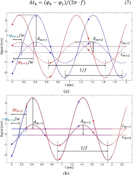
in all bursts would share the same frequency; features within the same burst would share a common phase; and the same features in different bursts would have the same amplitude and mean signal value (see Figure 5a). The other assumption is that the frequency of the signal is known nominally. If the total number of bursts is , this approach will reduce the total number of unknowns from 4� ∙ to � + + , and the design matrix for the adjustment will have the columns shown in Figure 6. After running this adjustment, the phase difference between any burst, , and the first one can be converted into a change in the time tag, ∆� , as shown in (7). Then, this time offset can be applied to the time tags of the bursts, and the signals for the available features in a particular burst can be superimposed over the ones from the first burst (see Figure 5b).
Δ� = � − � / � ∙ � (7)
(a)
(b)
Figure 5. Example of two bursts with a common frequency (1 Hz), but different phase, where the same two features in the different bursts have the same amplitude and mean signal value (a); the two bursts superimposed after applying the phase shift as to show the de-facto increase in the sampling frequency from 1.5 Hz to 3 Hz (b)
� � … � … … � �
Figure 6. The unknowns for a sinusoidal fitting adjustment combining multiple bursts
Other than reducing the total number of unknowns and thus increasing the redundancy of the solution, this methodology will also effectively increase the sampling frequency of the system at the cost of only one unknown (� ) per burst (see Figure 5b). Note that due to the strengthening of the geometry, this method will work reliably even if the original sampling frequency does not meet the Nyquist sampling requirement. The adjustment will converge to the correct solution as long as there is reasonable a-priori information about the frequency of loading.
3. DESCRIPTION OF LABORATORY SETUP AND CONDUCTED TEST
This section describes the laboratory environment and the tested specimen. It also lists the technical specifications of the components used in the photogrammetric system. Furthermore, details are given on the conducted test regiment, including the type of loading, its frequency and the corresponding camera exposure settings.
3.1 Laboratory Setup
A hydraulic actuator was installed in a structures laboratory and it was used for a beam deformation experiment. The actuator had a capacity of 250 kN, and was suspended from a steel cross beam, which was supported by two steel columns bolted to a 0.5 m thick concrete floor. The concrete beam to be tested (dimensions of 3 m x 300 mm x 150 mm) was painted white, and had a steel reinforced polymer sheet glued to its bottom. It was placed under the actuator, which applied a single point load (see Figure 7).
Figure 7. Experiment setup showing the hydraulic actuator and the concrete beam specimen
In addition to the actuator supporting frame, another steel frame was built around the actuator in order to hoist the components of the photogrammetric system in secure positions above the beam. The purpose of the photogrammetric system was to estimate the deformations of the top and bottom surfaces of the beam. Thirteen 150 mm x 50 mm or 150 mm x 75 mm thin aluminium plates painted in white were glued on the side of the beam (see Figure 8a). The plates served as offset witnesses to the bottom surface of the beam. Thus, the objects of interest for the photogrammetric system were the visible portions of the top surface of the beam and these offset witness plates. In order to be able to evaluate the accuracy of the photogrammetric system, five laser transducers were used as control sensors. An example ISPRS Annals of the Photogrammetry, Remote Sensing and Spatial Information Sciences, Volume III-5, 2016
of the laser transducers can be seen in Figure 8b. The laser transducers were operating at a sampling frequency of 120 Hz, and their overall precision had been previously evaluated to be approximately 10-30 µm.
(a) (b)
Figure 8. Close-up of two of the offset/witness plates (a), and one of the laser transducers (b)
3.2 Photogrammetric System Description
The photogrammetric system used for this project consisted of eight cameras and two projectors placed on one of the steel frames. The sensors were pointed normal to the top surface of the beam and the offset witness plates (see Figure 7). The make and model for the cameras was Canon EOS 1000D or Rebel XS. These cameras fall within the entry level DSLR category. Each camera had a 22.2 mm x 14.8 mm complementary metal oxide semiconductor (CMOS) solid state sensor. The output images had a maximum resolution of 10.1 mega pixels (i.e., 3888 pixels in width and 2592 pixels in height), where the pixel size was 5.71 µm. According to the manufacturer’s specifications, the cameras supported continuous shooting of up to three frames per second (fps). They were configured and synchronized (to 5 milliseconds) so that non-blurred images of both static and kinematic objects could be taken simultaneously. The synchronization was done through a hardware trigger (i.e., a wired remote control) connected to a hub, which could split the shutter release signal to all eight cameras. The make and model for the projectors was BenQ MP522 ST. These were short-throw projectors using single-chip light processing (DLP) technology, and their extended graphics array (XGA) had a resolution of 1024 pixels x 768 pixels. The projectors were used to display a pattern should artificial texture be necessary for the 3D reconstruction process of the observed surfaces/features. The photogrammetric system was calibrated in-situ once the cameras were pointed toward and focused on the beam. For this project the zoom rings of the camera lenses were set between 22 and 28 mm. Additionally, the image stabilization, automatic focus, and sensor cleaning functions of the cameras were disabled so the IOPs were as stable as possible.
3.3 Conducted Test Routine
A multi-day beam deformation experiment was conducted in three phases:
1. Phase I – static loading to settle the beam on its support; 3 mm displacements were applied at a rate of 1 mm per minute;
2. Phase II – static loading to initiate cracks in the specimen; a maximum load of 60 kN was applied at a rate of 3 kN per minute;
3. Phase III – dynamic loading, i.e., cycling between an expected low (e.g., 24 kN) and high (e.g., 72 kN) loads at a rate of either 1 Hz or 3 Hz.
Phase III was run until the beam reached failure, i.e., the polymer sheet separated from the bottom of the beam, the reinforcing rebar inside the beam fractured, and the beam experienced significant cracking. Image data was collected at zero load/displacement before the experiment commenced, during the three phases of the experiment, and after the end of the experiment for documenting the permanent damage. The focus of this paper will be the data collected during the 1 Hz and 3 Hz dynamic loading phase. The data consisted of multiple back-to-back bursts of still images, which lasted about ten seconds or 25-30 epochs. The 1 Hz images were collected at 1/15 of a second shutter speed and ISO of 100, while the 3 Hz images were collected at 1/60 of a second and ISO of 400. The approximate sensor frame rates were 2.52 and 2.87 fps, respectively (Detchev et al., 2014a).
4. MODEL-BASED IMAGE FITTING FOR 3D POSITIONING OF RECTANGULAR FEATURES
Once a point cloud of the concrete beam was reconstructed for each observation epoch, an image/point cloud processing algorithm was used to acquire the coordinate list for the offset witness plates. It is referred to as model-based image fitting, and it recovers the position of rectangular features in all three dimensions (Kwak et al., 2013).
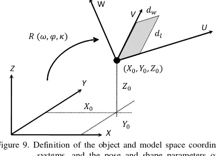
Model-based reconstruction uses the translation of a reference point ( , , ) and the rotation (�, �, �) of the model in object space (e.g., pose parameters), and the shape and size of the used primitive (e.g., shape parameters) to describe the object of interest. In the case of a rectangular target/plate, the shape can be defined by its width, �, and length, , dimensions. The model has its own coordinates system ( , , ). The origin is at the reference point (e.g., the lower left corner of the object), the and axes are aligned along the sides of the rectangle, and the axis is normal to the surface of the rectangle (see Figure 9). The relationship between the model coordinates of the rectangle vertices and their object space equivalents are expressed in equation (8):
Figure 9. Definition of the object and model space coordinate systems, and the pose and shape parameters of a rectangular model (after Kwak et al. (2013))
[ ] = [ ] + � �, �, � [ ] (8)
where is a function of the and coordinates of the reference point and the plane parameters , and :
= ∙ + ∙ + (9)
while � and � are defined using the orientation normal to the planar surface.
Since some of the model parameters (e.g., , , �, �) are only known approximately, an iterative adjustment procedure is implemented to finalize them. The adjustment minimizes the normal distance, , between the projected model and its realization in image space (see Figure 10). The realization of the model in the imagery is the model’s bounding edges derived through the Canny edge detector (Canny, 1986). It should be noted that each model was simultaneously adjusted in as many images as it appeared in, which increased the redundancy and thus the reliability of the solution (Kwak et al., 2013).
Figure 10. Projected rectangular model (before and after the model-based image fitting adjustment) and its relationship to a sample of detected edge pixels for one of the model sides (after Kwak et al. (2013))
5. EXPERIMENTAL RESULTS AND DISCUSSION
The , , and values derived from the model-based image fitting algorithm were run in the sinusoidal fitting adjustments as either separate models, combined models within a single burst or multiple back-to back bursts (see Table 1 to Table 6).
Precision Table 1. Statistical values for the sinusoidal fitting parameters
estimated for (1 Hz) Table 2. Statistical values for the sinusoidal fitting parameters
estimated for (1 Hz)
Note that while the new types of adjustments converged without any problems, the single model adjustments, especially for the 3
Hz data, had to sometimes be re-run several times until they converged to the correct solution. So when it comes to the single model adjustments, all the tables show their final results.
Precision Table 3. Statistical values for the sinusoidal fitting parameters
estimated for (1 Hz) Table 4. Statistical values for the sinusoidal fitting parameters
estimated for (3 Hz) Table 5. Statistical values for the sinusoidal fitting parameters
estimated for (3 Hz) Table 6. Statistical values for the sinusoidal fitting parameters
estimated for (3 Hz)
It should be noted from the tabulated results that the percentage goodness of fit, especially for and , increased for the newly proposed adjustments. Furthermore, the standard deviations for the frequency and phase parameters improved by one or two orders of magnitude. The standard deviations for the amplitude and the mean signal value also improved almost two-fold from the adjustment with one burst to the one including three bursts. ISPRS Annals of the Photogrammetry, Remote Sensing and Spatial Information Sciences, Volume III-5, 2016
Both improvements in the standard deviations were due to strengthening of the geometry by increasing the redundancy in a single adjustment. Finally, the correlation value between the frequency and phase went from 86% for the single burst adjustment to 48-71% for the three-burst one.
The repeatability in the estimation of the amplitude for the offset witness plates was also evaluated (see Table 7 and Table 8). The three different adjustments yielded similar results as the mean value (or the bias) and the root mean squared error (RMSE) of the differences between them was either at the RMSE level of the residuals or most of the time one order of magnitude smaller. So the assumption made in sections 2.3.1 and 2.3.2 proved to be valid.
Amplitude differences
One burst vs single model
Three bursts vs single
model
Three bursts vs one burst
Mean [mm] -0.003 0.004 0.007
RMS [mm] 0.006 0.006 0.010
Mean [mm] 0.005 0.005 0.000
RMS [mm] 0.017 0.030 0.025
Mean [mm] -0.003 -0.004 -0.002
RMS [mm] 0.005 0.007 0.005
Table 7. Bias and RMSE of the estimated amplitude values between the different adjustments (1 Hz)
Amplitude differences
One burst vs single model
Three bursts vs single
model
Three bursts vs one burst
Mean [mm] 0.000 0.003 0.004
RMS [mm] 0.004 0.014 0.015
Mean [mm] -0.003 -0.021 -0.018
RMS [mm] 0.011 0.040 0.034
Mean [mm] 0.008 -0.002 -0.010
RMS [mm] 0.022 0.035 0.023
Table 8. Bias and RMSE of the estimated amplitude values between the different adjustments (3 Hz)
Since five of the 13 plates were also observed by the control laser transducers, the mean (or bias) and RMSE values for the estimated plate amplitudes between the two systems were computed as well (see Table 9 and Table 10).
Accuracy quantities
Single
model One burst
Three bursts
Mean [mm] 0.019 0.023 0.015
RMSE [mm] 0.036 0.039 0.034
Table 9. Bias and RMSE of the estimated amplitudes between the photogrammetric system and the laser transducers (1 Hz)
Accuracy quantities
Single
model One burst
Three bursts
Mean [mm] 0.010 0.009 0.007
RMSE [mm] 0.070 0.066 0.071
Table 10. Bias and RMSE of the estimated amplitudes between the photogrammetric system and the laser transducers (3 Hz)
Again, the RMSE values (especially for the 1 Hz data) were at the same level as the RMSE values for their respective residuals. The RMSE values for the amplitude differences were also consistent across the three types of adjustments. The decrease in accuracy for the 3 Hz data could be attributed to the presence of more noise in the images acquired at ISO of 400 as opposed to 100.
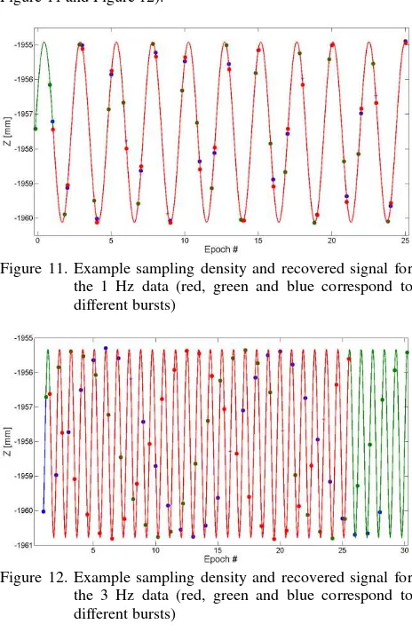
After the sinusoidal fitting adjustments for multiple bursts were run, the time offsets for the bursts were computed as was previously shown in (7). This way the data points and the recovered signals for the bursts could be plotted together (see Figure 11 and Figure 12).
Figure 11. Example sampling density and recovered signal for the 1 Hz data (red, green and blue correspond to different bursts)
Figure 12. Example sampling density and recovered signal for the 3 Hz data (red, green and blue correspond to different bursts)
This effectively increased the sampling rate of the camera system from 2.52 fps to 7.56 fps for the 1 Hz data, and from 2.87 fps to 8.61 fps for the 3 Hz data. This was especially crucial for the 3 Hz data. As seen in Figure 12, the separate red, green or blue data points define aliased signals; however, combined they describe the true specimen response to the applied loading test.
6. CONCLUSIONS AND RECOMMENDATIONS FOR FUTURE WORK
This paper introduced a new type of adjustment for performing sinusoidal fitting. The data handled was either single or multiple bursts coming from a photogrammetric system used for the 3D monitoring of a concrete beam. The specimen underwent dynamic/fatigue load testing at either 1 Hz or 3 Hz. The RMSE of the adjustment residuals ranged from 30 to 80 µm. The traditional and the new ways of estimating the amplitude of the ISPRS Annals of the Photogrammetry, Remote Sensing and Spatial Information Sciences, Volume III-5, 2016
specimen movements differed at the 5 to 30 µm level, which was either at or below the system noise. Also, compared to the amplitudes computed with data from the control laser transducers, the 1 Hz amplitude estimates were good to 40 µm, while the 3 Hz were good to 70 µm.
While all three methodologies yielded compatible results, the new adjustments were more reliable as they always converged to the correct solution. The new adjustments strengthened the geometry of the solution by decoupling some of the existing parameter correlations, and thus improved the standard deviations of the estimated parameters with up to two orders of magnitude (almost two-fold for the amplitude specifically). Moreover, by using three back-to-back bursts of data, it was shown that the effective sampling of the system was increased three-fold, which was especially beneficial for the otherwise aliased data collected during the 3 Hz loading.
Future work will include estimating the vertical deflections of the beam using the available portions of its top surface. The height/depth coordinates from the top surface of the beam will also be run in the new sinusoidal fitting adjustment.
ACKNOWLEDGEMENTS
The authors would like to thank Mohammad Moravvej, Dr. Hervé Lahamy, Jeremy Steward, Dr. Eunju Kwak and Kaleel Al-Durham for their support.
LIST OF REFERENCES
Brigham, E.O., 1988. The fast Fourier transform and its applications. Prentice Hall, Inc., Eaglewood Cliffs, New Jersey. Brownjohn, J.M.W., 2007. Structural health monitoring of civil infrastructure. Philosophical Transactions of the Royal Society A: Mathematical, Physical and Engineering Sciences 365, 589– 622.
Canny, J., 1986. A Computational Approach to Edge Detection.
IEEE Transactions on Pattern Analysis and Machine Intelligence PAMI-8, 679–698.
Detchev, I., Habib, A., El- Badry, M., 2013. Dynamic beam deformation measurements with off-the-shelf digital cameras.
Journal of Applied Geodesy 7, 147–157.
Detchev, I., Habib, A., He, F., El-Badry, M., 2014a. Deformation monitoring with off-the-shelf digital cameras for civil engineering fatigue testing, International Archives of the Photogrammetry, Remote Sensing and Spatial Information Sciences, Vol. XL(5), pp. 195–202.
Detchev, I., Mazaheri, M., Rondeel, S., Habib, A., 2014b. Calibration of multi-camera photogrammetric systems, The International Archives of the Photogrammetry, Remote Sensing and Spatial Information Sciences, Vol. XL(1), pp. 101–108.
Fraser, C.S., 1997. Digital camera self-calibration. ISPRS Journal of Photogrammetry and Remote Sensing 52, 149–159. Fraser, C.S., Riedel, B., 2000. Monitoring the thermal deformation of steel beams via vision metrology. ISPRS Journal of Photogrammetry and Remote Sensing 55, 268–276.
Gordon, S.J., Lichti, D.D., 2007. Modeling Terrestrial Laser Scanner Data for Precise Structural Deformation Measurement.
Journal of Surveying Engineering 133, 72–80.
Habib, A.F., Morgan, M.F., 2003. Automatic calibration of low-cost digital cameras. Optical Engineering 42, 948–955. Harris, C., Stephens, M., 1988. A combined corner and edge detector. Presented at the 4th Alvey Vision Conference, Manchester, UK, pp. 147–151.
Jáuregui, D.V., White, K.R., Woodward, C.B., Leitch, K.R., 2003. Noncontact Photogrammetric Measurement of Vertical Bridge Deflection. Journal of Bridge Engineering 8, 212–222. Jiang, R., Jáuregui, D.V., 2007. A Novel Network Control Method for Photogrammetric Bridge Measurement.
Experimental Techniques 31, 48–53.
Jiang, R., Jáuregui, D.V., White, K.R., 2008. Close-range photogrammetry applications in bridge measurement: Literature review. Measurement 41, 823–834.
Kwak, E., Detchev, I., Habib, A., El-Badry, M., Hughes, C., 2013. Precise Photogrammetric Reconstruction Using Model-Based Image Fitting for 3D Beam Deformation Monitoring.
Journal of Surveying Engineering 139, 143–155.
Lichti, D.D., Jamtsho, S., El-Halawany, S.I., Lahamy, H., Chow, J., Chan, T.O., El-Badry, M., 2012. Structural Deflection Measurement with a Range Camera. Journal of Surveying Engineering 138, 66–76.
Lichti, D.D., Stewart, M.P., Tsakiri, M., Snow, A.J., 2000. Calibration and testing of a terrestrial laser scanner. International Archives of Photogrammetry and Remote Sensing Vol. XXXIII, 485–492.
Maas, H.-G., Hampel, U., 2006. Photogrammetric techniques in civil engineering material testing and structure monitoring.
Photogrammetric Engineering & Remote Sensing 72, 39–46. Mills, J.P., Newton, I., Peirson, G.C., 2001. Pavement Deformation Monitoring in a Rolling Load Facility. The Photogrammetric Record 17, 7–24.
Park, H.S., Lee, H.M., Adeli, H., Lee, I., 2007. A New Approach for Health Monitoring of Structures: Terrestrial Laser Scanning. Computer-Aided Civil & Infrastructure Engineering
22, 19–30.
Qi, X., Lichti, D.D., El-Badry, M., Chan, T.O., El-Halawany, S.I., Lahamy, H., Steward, J., 2014a. Structural Dynamic Deflection Measurement With Range Cameras. Photogram Rec
29, 89–107.
Qi, X., Lichti, D., El-Badry, M., Chow, J., Ang, K., 2014b. Vertical Dynamic Deflection Measurement in Concrete Beams with the Microsoft Kinect. Sensors 14, 3293–3307.
Rönnholm, P. et al., 2009. Comparison of measurement techniques and static theory applied to concrete beam deformation. The Photogrammetric Record 24, 351–371. Whiteman, T., Lichti, D.D., Chandler, I., 2002. Measurement of deflections in concrete beams by close-range digital photogrammetry. The Symposium on Geospatial Theory, Processing and Applications, Ottawa, Canada.