TOWARDS FAST MORPHOLOGICAL MOSAICKING OF HIGH-RESOLUTION
MULTI-SPECTRAL PRODUCTS – ON IMPROVEMENTS OF SEAMLINES
Tobias Storch, Peter Fischer, Sebastian Fast, Philipp Serr, Thomas Krauß, Rupert Müller
German Aerospace Center (DLR), Earth Observation Center (EOC), Münchener Str. 20, 82234 Weßling, Germany [email protected]; [email protected]; [email protected]; [email protected];
[email protected]; [email protected]
KEY WORDS: Optical Remote Sensing, High-Resolution Product, Mosaic, Morphological Image Processing, Seamline, Quasi-Linear Runtime
ABSTRACT:
The complex process of fully automatically establishing seamlines for the fast production of high-quality mosaics with high-amount of high-resolution multi-spectral images is detailed and improved in this paper. The algorithm is analyzed and a quasi-linear runtime in the number of considered pixels is proven for all situations. For typical situations the storage is even essentially smaller from a complexity theoretical perspective. Improvements from algorithm practical perspective are specified, too. The influence of different methods for the determination of seamlines based on gradients is investigated in detail for three Sentinel-2 products. The studied techniques cover well-known ones normally based on a single band. But also more sophisticated techniques based on multiple bands or even taking additional external geo-information data are taken into account. Based on the results a larger area covered by Image2006 orthorectified products with data of the Resourcesat-1 mission is regarded. The feasibility of applying advanced subordinated methods for improving the mosaic such as radiometric harmonization is examined. This also illustrates the robustness of the improved seamline determination approaches.
1. INTRODUCTION
1.1 Mosaicking of High-Resolution Multi-Spectral Images
For analysis of larger areas it is often necessary to synthetically combine multiple small area products to one single product covering a large spatial extent. This is necessary, e.g., because of a small swath or a high cloud coverage. The joining of data is relevant to optical and radar as well as to spaceborne and airborne acquisitions. Beside Earth observation the merging is also a relevant discipline, e.g., in planetary sciences. And mosaicking applies to data of all spectral and spatial resolutions. Even combining products from different missions and instruments is accounted for in remote sensing (Szeliski 2006).
In this paper we focus on high-resolution multi-spectral Earth observation imagery that is orthorectified. And all considered products share similar characteristics, namely spatial resolutions in the order of 10 m and spectral divisions in the order of 10 bands in the visible, near and short-wave infrared. Here, experiments were performed using data from Sentinel-2/MSI and Resourcesat-1/LISS III.
A correction of the co-registration error between products is not considered, here. It is assumed that the co-registration error between the products is in the order of lower than one pixel. However, the combination of images still has to account for several challenges, e.g., inhomogeneous radiometry such as illumination conditions, different content such as changed agriculture or forestry, and undesired objects such as clouds in the images (Bignalet-Cazalet et al. 2012).
Two major strategies for combining data are typically distinguished. Namely, each pixel of the mosaic represents the pixel value of either one of the overlapping input images – called best-pixel approach – or a combination of the pixels of the overlapping input images – called mixed-pixel approach. Many algorithms, e.g., for classification of land cover and land usage (Cihlar 2000), rely on the physical measurement of each
pixel. And therefore, we focus on the best-pixel approach in the following.
The selection of the unique pixel is either performed for each pixel independently or considering regions of connected pixels. Numerous algorithms consider neighboring pixels, where the same acquisition conditions are favorable. And therefore, we focus on considering regions of connected pixels. In this situation it is desirable to minimize the number of changes between regions of the different images involved. The lengths of the lines between regions are of minor importance.
Hence, taking two or more overlapping images into account, the challenge is to determine a seamline or seamlines between these images (Yu et al. 2012). There exist several methods to determine seamlines. Due to the high number of products to be considered, especially for European or even global coverages, we focus on fully automatic algorithms. We even focus on algorithms with quasi-linear runtime complexity in the number of pixels that serve as input and output. Therefore, popular graph-based algorithms for seamline determination are not considered as they need at least cubic runtime complexity since they optimize a maximum flow (Fernandez et al. 1998). A popular quasi-linear (or also called log-linear) runtime algorithm realizing high-quality mosaics is the morphological image compositing/mosaicking by Soille (2006). It was established for similar types of products. We consider further improvements of the most critical step of the heuristic, namely the robust determination of seamlines. Such investigations are not in the focus of publications so far concerning morphological image compositing/mosaicking. This is also true for the in more detail considered runtime and storage complexity.
1.2 Sentinel-2 and Image2006 Products
Orbit SSO, 10:30 SSO, 10:30
Instrument MSI LISS III
Spectral Resolutions and Ranges
blue, green, red, near infrared; vegetation red edge (4 bands),
shortwave infrared (2 bands); aerosol,
water-vapor, cirrus
green, red, near infrared,
shortwave infrared
Spatial Resolutions and Swaths
10 m; 20 m; 60 m at 290 km
20 m (resampled from 23.5 m)
at 141 km Geolocation
Accuracies
Abs.: 20 m (3σ), Rel.: 0.3 px (2σ)
Abs.: 13 m (1σ), Rel.: 0.5 px (1σ)
Table 1. Missions overview.
It has to be remarked that the number of overlaps equals 1,232 for the 109 considered products of Image2006.
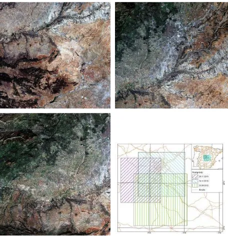
An overview of the considered Sentinel-2 products is given in Figure 1. Figure 2 illustrates the footprints of the considered Image2006 products.
Figure 1. Chronologically sorted true color quicklooks of three Sentinel-2 products of Madrid, Spain, and their footprints.
1.3 Structure of the Paper
After this introduction in section 1, we illustrate the complete process of morphological image mosaicking considered in section 2 with an overview and details on the processing steps
Figure 2. Footprints with degree of overlap of 109 Image2006 products (based on Resourcesat-1) of France.
2. PROCESS OF MORPHOLOGICAL IMAGE MOSAICKING
2.1 Overview
For the considerations of runtime and storage complexities we state them with respect to the number of pixels and with respect to the input image and output mosaic – and considering additionally the number of images for investigations of storage. We refer to Wegener (2005) for definitions of notations and complexities. (Roughly speaking a = O(b) can be read as a is at most of the same order as b.)
Let us assume that a mosaic of m pixels shall be generated based on k input images with the same map projection and spatial (and spectral) resolution of n pixels in total.
Based on a marker mosaic the mosaic is produced by pixel-based insertion of the pixel of the indexed input image to the mosaic. In the marker mosaic for each pixel of the mosaic the index of the contributing input image is contained (each index of 0,1,…,k is stored with O(log k) bits). Thus, the mosaic is produced in linear runtime O(m) and the marker mosaic needs storage O(m log k). The mosaic itself needs storage O(m). Therefore, we only investigate the generation of the marker mosaic in the following.
In case that different spatial resolutions apply for different spectral bands of a product, the marker mosaic is established on the either
• worst spatial resolution which guarantees that each spectral profile represents a physical measurement or
• best spatial resolution, where the pixel for worse spatial resolution is chosen based on a majority vote of the underlying best spatial resolution pixels which guarantees that a high-quality seamline is determined for the best spatial resolution.
Figure 3. Illustration of the process of morphological image mosaicking.
1. Initializing. [Set up major data structures.]
2. Identifying Overlaps. [Set feasible contributions of each input image to the marker mosaic. E.g., Figure 4.a.]
3. Determining Markers including Determination of Gradients for Seamlines. [Assume indices for all pixels in the marker mosaic with a lower degree of overlap than considered degree of overlap are already set fixed. Set indices for edge pixels in the marker mosaic with the considered degree of overlap to a lower degree of overlap. The indices are taken from the pixels of lower degree of overlap. E.g., Figure 4.b and 4.c.]
4. Growing Markers including the Determination of Gradients for Seamlines. [Flood the indices of edge pixels in the marker mosaic to its neighbors of the same overlap with a marker-based watershed transformation based on a gradient image as elevation model. The indices are taken from the neighbor pixels. E.g., Figure 4.c and 4.d.]
The resulting process of setting the markers is exemplarily illustrated in Figure 4 based on the three Sentinel-2 products of Madrid, Spain.
We will observe, that the runtime to generate the marker mosaic is bounded by O(m log m + n). Assuming reasonably that m = O(n) the runtime is bounded by O(n log n), namely it is a quasi-linear (or also called log-quasi-linear) runtime algorithm. The storage is bounded by O(m·(k + log m) + n). Or it is O(m·(k + log m)) by not taking the storage for input into account. And with the assumption k is small – e.g., k = O(log n) – the storage is bounded by O(m log n).
Figure 4. Degree of overlap, where degree 0:white, 1:green, 2:blue, and 3:orange in a. Illustrating the determination and growing markers with degree of overlap 1 in b., 2 in c., 3 in d.
However, by using hash tables (Knuth (1998) and marked with [Hash Table] in the following subsections) the storage is potentially reduced. E.g., if the number of non-empty overlaps of input images is O(log n) and the size of a largest overlap in pixel is O(m/log n), the storage is bounded by O(m log log n + n). This is even needed to store the marker mosaic. And the runtime remains O(n log n).
Furthermore, it is easy to modify the algorithm such that the insertion and removal of an image to the mosaic (not changing its size) can be realized in quasi-linear runtime with respect to the number of pixels of the input image. Also the masking of undesirable regions, e.g., cloudy or hazy regions, can be realized by assigning the pixels as background.
2.2 Initializing
The marker mosaic shall be initialized with zero for each pixel in runtime O(m). This is based on the metadata of the input images containing their geographical coverage or based on a defined area of interest. Each pixel of the marker mosaic shall additionally contain a bit-string of length k and a state {0;1}. The data structure needs storage O(mk). After the processing step of identifying overlaps the bit-string shall indicate all indices of input images which cover the corresponding pixel. The state indicates if the corresponding pixel was already considered in the processing steps of determining (state changes to 1) and growing (state changes to 0) markers. The data structure shall be initialized with zeros for the bit-string and with zero for the state for each pixel in runtime O(m).
Let us discuss the following improvements to this basic concept.
O(log s) = O(min{k;log m;log n}) for a pointer to the set in the hash table.
• In order to practically increase especially the parallel computation performance the mosaic can be tiled in smaller portions.
2.3 Identifying Overlaps
To identify overlaps with information of the input images which overlap, we perform the following for each pixel (not being background or not being considered anyhow) of each input image (in arbitrary order). Let i be the index of the input image. Set the i-th position of the bit-string from zero to one in runtime O(1). And set the pixel of the marker mosaic to i. Finally, we have identified all overlaps and all pixels of the marker mosaic are set. The step of identifying overlaps is performed in runtime O(n) in total.
• [Hash Table] If the pixel of the marker mosaic points to set S, it shall point to set S ᴗ {i}. Due to the properties for look-ups and insertions in hash tables, this is performed in runtime O(1) in average for each pixel and in runtime O(n) in total.
• The step of identifying overlaps can be parallelized input image- and pixel-based.
2.4 Determining Markers
To determine markers we perform the following for each degree d of overlap (in increasing order) for each pixel of the marker mosaic (in arbitrary order). We consider the 4- and 8-neighborhood, but the method is directly to adapt to other definitions of neighborhood. If the degree of overlap for the pixel equals d, set the state of the pixel to 1. For each pixel which state was changed,
• from the multiset of indices of neighbor pixels remove all indices i,
o where i = 0, namely are background or not being considered anyhow,
o where the bit-string of the pixel does not contain i, namely the pixel is not allowed to be set to i, (e.g., two overlaps with degree one hit together) and
o where the bit-string of the neighbor pixel represents a set of size at least d, namely the method is independent to the order of pixels considered (e.g., set during the processing step of identifying overlaps to guarantee that indices of pixels with degree of overlap lower than d are surely set),
and let v be the maximum of all remaining indices in the multiset that represent the maximum occurrences or, if the multiset is empty, let v be 0, where pixels with v ≠ 0 are called marker pixels,
• if v ≠ 0,
o set the state of the pixel to 0 and its index to v and
are even determined in O(1). We establish a bounded capacity priority queue (Knuth 1998) with a constant number of priorities in runtime O(1). When the recursion terminates for a pixel, for a complete overlap all markers at edges to overlaps with a lower degree of overlap are contained in the priority queue. A complete overlap consists of all neighboring pixels with the same bit-string. And all states are set to 1. Perform the processing step of growing markers for the initialized priority queue. Finally, all markers are set. In general, the priority queues need storage O(m log m). Since the size r of complete overlaps in pixel is typically small, e.g., r = O(m/log m), also the needed storage is with O(r log m) much smaller, e.g., O(m). Thanks to the initialization of the marker mosaic in the processing step of identifying overlaps, it is sufficient to consider d ≥ 2.
• In order to practically increase especially the parallel computation performance and taking swapping effects into account, the complete overlap – which is typically roughly rectangular – is estimated in dimension, the gradients are determined, as well as the markers are determined and grown.
2.5 Growing Markers
To grow markers we perform the following until the priority queue is empty. The bounded capacity priority queue shall be realized in a first-in-first-out manner as discussed in the next section. For each pixel pointed to by the priority queue, set its state to 0. The indices of these marker pixels are already set appropriately. Remove the first pointer of the lowest non-empty priority in runtime O(1). Let the index of the considered pixel be denoted by v that is pointed to. For all its neighbor pixels that are in state 1 and have the same bit-string as the considered pixel,
• set the state of the neighbor pixel to 0 and its index to v and
• insert a pointer to the pixel to the priority queue assigned with the value of the gradient which is determined according to section 3 as priority.
This is performed in runtime O(log m) assuming that the gradient is determined in O(log m) as well. We observe that finally a marker-based watershed transformation is realized (Vincent et al. 1991) with the gradients as elevations. Consider each pixel of the marker mosaic. For at most one value of d the pixel is inserted and removed from the priority queue during determining or growing markers. This is performed in runtime O(log m). For each of the other values of d, which are at most k – 1, runtime O(1) is needed. The steps of determining and growing markers are performed in runtime O(m log m) in total.
• [Hash Table] The runtime for the step of determining and growing markers is not (significantly) affected by using hash tables.
3. DETERMINATION OF GRADIENTS FOR SEAMLINES
3.1 Overview
In this section the small area detailed analysis covered by three Sentinel-2 Level 1C products is carried out.
We will first discuss that the gradient is always simply set to a constant value. If the priority queue is realized in a last-in-first-out manner, a constant setting of the gradients results in a marker mosaic based on stacking of the input images. This is, e.g., prioritized according to the date, if the indices of the input images are set appropriately. We observe that the result is already obtained when stopping after the processing step of identifying overlaps. If the priority queue is realized in a first-in-first-out manner, a constant setting of the gradients results in a marker mosaic based on Voronoi segmentation. Results for stacking and Voronoi segmentation are illustrated in Figure 5. In the next subsections gradients are considered based first on a single band and second on multiple bands. The consideration of additional external data such as geo-information products of streets is carried out afterwards. E.g., to cope with co-registration errors the application of filters is taken into account. Finally, an optimal configuration for the determination of gradients for seamlines is identified and considered for a larger area in the next section.
Figure 5. True color mosaic of the three Sentinel-2 products of Madrid, Spain, based on stacking (left) and Vornoi
segmentation (right).
3.2 Based on Single Bands
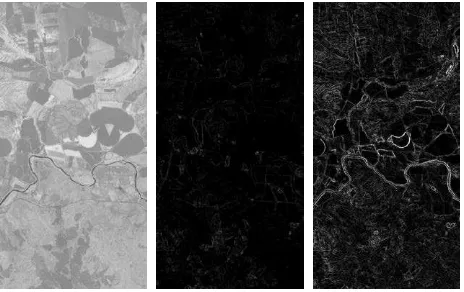
Let us consider the situation that a gradient is computed by applying the Scharr operator (Jähne et al. 1999) on a single band image with a radiometric quantization of 8-bits. The effects are similar for the Sobel operator or other edge detection operators. This results in gradients holding gray values between 0 and 255. The consideration of gradients based only on single bands results in multiple challenges. As shown in Figure 6 contours are highly dependent on the data contrast and quality. E.g., gradients only based on the blue bands or the near infrared bands tend to be not reliably solid and constant. This is even true if the utilization of the near infrared band is superior to the blue band, here. However, the methods should reliably discover such contours, e.g., farmlands, streets, or rivers, but gradients based on single bands typically lead to unrepresentative objects. Let us consider that an overlap is covered by multiple input images. Since for each input image its own gradients are generated, namely multiple gradients for each pixel exist, they have to be aggregated to a final gradient. In order to account for structures common in all input images of the overlap, the pixel-based minimum is selected as final gradient.
Figure 6. NDVI quicklook of the region of the three Sentinel-2 products of Madrid, Spain, under consideration (left) as well as gradient image based on blue band (middle) and near infrared
band (right).
3.3 Based on Multiple Bands
Due to the lack of precision of single band gradients, multiple band gradients are considered. E.g., the maximum of the final gradients for each band is considered. Here, special focus is given to the Normalized Differenced Vegetation Index (NDVI) (Ogashawara et al. 2012). The NDVI is probably the widest recognized index and provides information how far the considered region contains live green vegetation or not. It is calculated via the ratio of a broad-band red band (0.6 µm to 0.7 µm) and a broad-band near infrared band (0.8 µm to 0.9 µm), namely
NDVI = (near infrared – red) / (near infrared + red).
As the NDVI detects differences in vegetation, it also recognizes differences between farmland, streets, and rivers. Farmland usually grows different crops and thus also reflects differently for each field. However, the NDVI is typically between 0.2 and 1.0. Streets are usually not vegetated and thus the NDVI is typically below 0.2 and so do rivers typically featuring negative NDVI. Considering the distinct uniqueness of farmland, streets, and rivers in the NDVI, such information helps to distinguish between suitable objects to use for generating gradients and also seamlines as illustrated in Figure 7.
Figure 7. NDVI quicklook of the region of the three Sentinel-2 products of Madrid, Spain, under consideration (left) as well as gradient image based on NDVI (middle) and resulting setting of
e.g., of streets and rivers in vector format of almost every country. Merging the road information from this data source with our existing gradient images emphasizes the already existing edges caused by the abrupt change between road and surrounding vegetation. In our experiments we found out that balance between image data and VGI has to be ensured. In regions covered by forest roads beneath the tree crowns are not visible in the mosaic, placing seamlines in such situations would be inappropriate. The same holds true for roads hidden by other objects, e.g., tunnels or crossed by another dominant entity like a river. There is no guarantee for the correctness and completeness of obtained data, e.g., concerning geo-location of streets or rivers, or data is not available at all. It is remarked that in the latter situation of no data a Voronoi segmentation is obtained. However, with this information typically straight, solid, and constant seamlines can be determined.
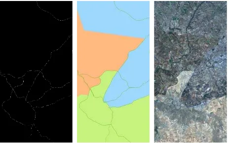
Figure 8 shows the vectored geo-information data, the gradient image generated from the rasterized geo-information data, the resulting segmentation of the images, and the mosaic itself.
Figure 8. Gradient image based on streets of the region of the 3 Sentinel-2 products of Madrid, Spain, under consideration (left) as well as the resulting setting of markers (middle) and the
resulting true color mosaic (right).
3.5 Filters
Typically filters are applied before the generation of the gradients of each image to remove noise or reduce effects due to co-registration errors, e.g., by the Gaussian filter. We discovered spikes and noise in the image of the NDVI which alters the gradient determination in an insufficient manner. Hence, we used particularly a Gaussian filter to blur the image of the NDVI prior to the gradient determination.
3.6 Optimized Segmentation
Seamlines determined based on gradients of images of NDVI may not be straight, but rather fuzzy, as illustrated in the previous section. To generate rather straight than fuzzy seamlines, one approach is to consider strengthening the
During rasterization of the vector format data of streets the (expected) spatial dimensions of the street, especially the (expected) number of lanes depending on the type of street, have to be considered as illustrated in Figure 9. They typically have widths different to exactly one pixel. When enhancing gradients with rasterized vector format data of streets, it is very important to only use types of streets that are applicable to the spatial resolution of the input image.
Figure 9 illustrates multiple approaches for optimizing gradients with rasterized vector format data of streets. Contours in gradients shall be gray values between 0 and 255 representing the contrast at the given position. However, typically images of gradients do usually not have predictable ranges of equally distributed gray values. They have spikes which represent extraordinary high or low values outlying the typical spectral distribution of gray values in the gradient. Streets are expected to have relatively solid contours, but their gray values range between 10% and 25% of the range. Because their spectral profile is not that predictable, it is rather difficult to merge rasterized vector data of streets with the gradients. The streets are mapped on the gradient considering its arithmetic average pixel value above zero. Most of the pixels are dark and as such the arithmetic average remains low. Ultimately, streets are removed from the gradient by considering this approach. The plot of the streets on the gradient considering its median pixel value is shown as well. The median is higher than the arithmetic average, because we have values representing the complete range of gray values. Finally, the gradient is multiplied pixel-based with a specific value representing the (expected) solidness of the street type is illustrated. E.g., motorways and trunk roads are multiplied by two, while primary roads are multiplied by one.
4. EXPERIMENTAL RESULTS 4.1 Overview
In this section a large area experimental investigation, covered by 109 orthorectified products of Image2006 which is based on data of the Resourcesat-1 mission, is carried out.
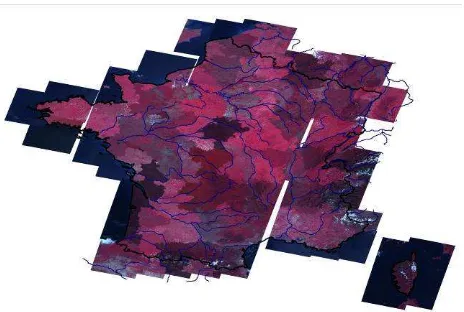
The size of the products is approximately 75 gigabyte with a size of approximately 21.1 giga-pixel (13.3 giga-pixel in France). Approximately 5.1 giga-pixel contribute to the final mosaic as illustrated in Figure 10.
Figure 9. Gradient image (left) and resulting true color mosaic (right) of the region of the three Sentinel-2 products of Madrid, Spain, under consideration, where the first row: NDVI, second
row: average, third row: median, forth row: majority.
4.2 Determination of Seamlines
Concerning the seamline determination we observed even in case of using just a single band that the seamlines mostly tend to follow dominant, landscape shaping entities, e.g., rivers or mountain ridge lines. As brightness differences between two images can be easily detected within an area of the same material, e.g., open soil and closed forest, this behavior is highly appreciated. Rivers and streets can act as borders between images. As the occurrence of brightness differences at these borders is expected, the generated seamlines are almost invisible in the final mosaic. The generated seamlines strongly depend on the used spectral information for creating the gradient image. In our experiments we also used multiple bands and indices to generate the gradient image. The most promising results were gained by using multiple bands in the red-edge domain, which are known to be very sensitive to changes between vegetation and other material. As in Figure 10 can be seen, rivers often serve not just as natural barriers, but also as seamlines in the final mosaic.
Figure 10. False color mosaic of the 109 Image2006 products of France, where major rivers are highlighted.
Beside of this, especially man-made objects are often detected as seamlines. Such objects like streets, roof tops, and other urban features are already well-known for serving as entrance points in different relative radiometric normalization techniques. Schott et al. (1988) gives a comprehensive overview about relative radiometric normalization. In this and subsequent works vegetation masks are often used to exclude such areas from the histogram matching process. It is pointed out that image features with a constant reflectivity serve best for determining the gain/offset values to adapt images to each other. The reliable identification of such pseudo-invariant features (PIF) between corresponding image pairs is thus the main challenge. This inspired us to use indices which suit for distinguishing between urban and non-urban image features. Simple indices like Normalized Differenced Vegetation Index (NDVI) which are based on band ratios already help to extract more suitable seamlines. Using freely available information about street networks strongly extends the purely image based approach to a new level. In non-urban areas such information supports the establishment of reliable image edges.
4.3 Radiometric Harmonization
The seamline detection focuses on regions with a constant reflectivity. Thus, in general the edge between images should be almost not visible. Nevertheless, we observed conditions when sharp edges arise in the final image. Typical error sources are a large temporal offset between image acquisition dates, changes in phenology, and changing weather conditions, e.g., due to clouds and haze. In contrast to these factors the influence of differing sun and viewing angles on radiometric stability is quite low. To overcome these problems, radiometric block adjustment as a processing step should be added. Examples are given by Angelo (2007).
4.4 Multi-Source Data Fusion
experiments carried out.
5. CONCLUSIONS
We analyzed an algorithm for image mosaicking of high-resolution orthorectified products, e.g., of the Sentinel-2 mission, based on morphological image processing which is especially fully automatic and highly efficient with a quasi-linear (also called log-quasi-linear) runtime. Such a runtime is a key factor for the timely provision of European or global mosaics. The quality of the image mosaic is probably strongest influenced by the gradient images used for seamline estimation. The major improvements by taking not only a single band into account as typically realized, but multiple bands combined with additional external geo-information data such as of the vectored street data is illustrated and discussed based on Sentinel-2 and Image2006 products.
Future work will consider the determination of gradients based, e.g., on land cover and land use, classification or cluster results that are estimated based on the images themselves – essentially combined with data of the OpenStreetMap project. The algorithm will be more strictly tailored to the specifications of the Sentinel-2 mission.
ACKNOWLEDGEMENTS
The authors thank the anonymous reviewers for their suggestions how to improve the paper.
REFERENCES
Angelo, P., 2007. Radiometric alignment and vignetting calibration. In: Proceedings of the ICVS Workshop on Camera Calibration Methods for Computer Vision Systems 2007, Bielefeld, Germany, pp. 1-10.
Baillarin, S.J., A. Meygret, C. Dechoz, B. Petrucci, S. Lacherade, T. Tremas, C. Isola, P. Martimort, F. Spoto, 2012. Sentinel-2 Level 1 Products and Image Processing Performances. In: The International Archives of the Photogrammetry, Remote Sensing and Spatial Information Sciences, Melbourne, Australia, Vol. XXXIX, Part B1, pp. 197-202.
Bignalet-Cazalet, F., S. Baillarin, C. Panem, 2012. Automatic and Generic Mosaicing of Multisensor Images: An Application to Pleiades HR. In: The International Archives of the Photogrammetry, Remote Sensing and Spatial Information Sciences, Melbourne, Australia, Vol. XXXIX, Part B1, pp. 509-512.
Academic Press.
Knuth, D.E., 1998. The Art of Computer Programming. Part 3: Sorting and Searching. Addison-Wesley.
Müller, R., T. Krauß, M. Schneider, P. Reinartz, 2012. Automated Georeferencing of Optical Satellite Data with Integrated Sensor Model Improvement. Photogrammetric Engineering and Remote Sensing, 78(1), 61-74.
Ogashawara, I., V. da Silva Brums Bastos, 2012. A Quantitative Approach for Analyzing the Relationship between Urban Heat Islands and Land Cover. Remote Sensing, 4, 3596-3618.
Roy, D.P., J. Ju, K. Kline, P.L. Scaramuzza, V. Kovalskyy, M.C. Hansen, T.R. Loveland, E.F. Vermote, C. Zhang, 2010. Web-enabled Landsat Data (WELD): Landsat ETM+ Composited Mosaics of the Conterminous United States, Remote Sensing of Environment, 114(1), 35-49.
Schott, J.R., C. Salvagio, W.J. Volchok, 1988. Radiometric scene normalization using pseudoinvariant features. Remote Sensing of Environment, 26(1), 1-26.
Soille, P., 2006. Morphological image compositing. IEEE Transactions on Pattern Analysis and Machine Intelligence, 28(5), 673-683.
Szeliski, R., 2006. Image alignment and stitching: A tutorial. Foundations and Trends in Computer Graphics and Vision, 2(1), 1-104.
Vincent, L., P. Soille, 1991. Watershed in digital spaces: An efficient algorithm based on immersion simulations. IEEE Transactions on Pattern Analysis and Machine Intelligence, 13(6), 583-598.
Wan, Y., D. Wang, J. Xiao, X. Lai, J. Xu, 2013. Automatic determination of seamlines for aerial image mosaicking based on vector roads alone. ISPRS Journal of Photogrammetry and Remote Sensing, 76, 1-10.
Wegener, I., 2005. Complexity Theory. Springer.