CLOUD PHOTOGRAMMETRY FROM SPACE
K. Zakšek a, *, A. Gerst b, J. von der Lieth a, G. Ganci c, M. Hort a
a
University of Hamburg, CEN, Institute of Geophysics, Bundesstr. 55, 20146 Hamburg, Germany – [email protected], [email protected], [email protected]
b
ESA, European Astronaut Centre, Linder Höhe, 51147 Köln, Germany C
INGV, Sezione di Catania, Piazza Roma, 2, 95125 Catania, Italy – [email protected]
KEY WORDS: photogrammetry, cloud top height, volcanic ash, SEVIRI, MODIS, ISS
ABSTRACT:
The most commonly used method for satellite cloud top height (CTH) compares brightness temperature of the cloud with the atmospheric temperature profile. Because of the uncertainties of this method, we propose a photogrammetric approach. As clouds can move with high velocities, even instruments with multiple cameras are not appropriate for accurate CTH estimation. Here we present two solutions. The first is based on the parallax between data retrieved from geostationary (SEVIRI, HRV band; 1000 m spatial resolution) and polar orbiting satellites (MODIS, band 1; 250 m spatial resolution). The procedure works well if the data from both satellites are retrieved nearly simultaneously. However, MODIS does not retrieve the data at exactly the same time as SEVIRI. To compensate for advection in the atmosphere we use two sequential SEVIRI images (one before and one after the MODIS retrieval) and interpolate the cloud position from SEVIRI data to the time of MODIS retrieval. CTH is then estimated by intersection of corresponding lines-of-view from MODIS and interpolated SEVIRI data. The second method is based on NASA program Crew Earth observations from the International Space Station (ISS). The ISS has a lower orbit than most operational satellites, resulting in a shorter minimal time between two images, which is needed to produce a suitable parallax. In addition, images made by the ISS crew are taken by a full frame sensor and not a push broom scanner that most operational satellites use. Such data make it possible to observe also short time evolution of clouds.
*
Corresponding author
1. INTRODUCTION
Information on height of clouds independent of their origin (natural or anthropogenic aerosol clouds, meteorological clouds) is important in different research fields. Cloud top height (CTH) is especially interesting for meteorologists. In some countries, like Midwest USA, a lot of effort is dedicated towards observation of convective clouds (Cumulonimbus) that might develop in so called super cells. Tops of such clouds can reach heights of over 20 km making them a source of dangerous severe weather, such as hail, heavy precipitation, or tornadoes (Heymsfield et al., 1983). Furthermore, the top cloud height is relevant for climatology, because the height is related to the amount of long-wave radiation that is emitted to space. Computing the heights for a part of the available data archives may extract some interesting climatological trends. Another important application is monitoring of aerosols produced in forest fires or industrial accidents (for instance explosions in chemical factories, oil refineries or power plants).
In this contribution, we focus on the volcanic ash heights because of the huge economic loss of the 2010 Eyjafjallajökull volcanic eruption. We knew already before that volcanic eruptions can have a significant impact on air traffic; between 1953 and 2009 Guffanti et al. (2010) report 128 encounters between aircraft and volcanic ash worldwide. The International Air Transport Association (IATA) stated that the total loss for the airline industry as a result of the airspace closure during the eruption of Eyjafjallajökull was around €1.3 billion (BBC News, 21/04/10): over 95,000 flights had been cancelled all across Europe during the six-day travel ban (BBC News, 21/04/10), with later figures suggesting 107,000 flights
2. STATE OF THE ART IN CTH ESTIMATION
Clouds can be observed from the ground by common weather radar or by atmospheric lidar that received increasing attention. Although these are excellent tools, all ground based measurements are restricted to their low spatial and temporal
availability. Compared to ground or airborne based observations satellite remote sensing provides global observations. In the table 1, we briefly review different satellite remote sensing techniques for aerosol / meteorological clouds height retrieval.
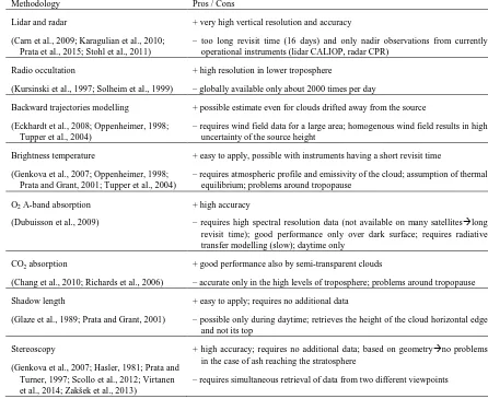
Methodology Pros / Cons
Lidar and radar
(Carn et al., 2009; Karagulian et al., 2010; Prata et al., 2015; Stohl et al., 2011)
+ very high vertical resolution and accuracy
– too long revisit time (16 days) and only nadir observations from currently operational instruments (lidar CALIOP, radar CPR)
Radio occultation
(Kursinski et al., 1997; Solheim et al., 1999)
+ high resolution in lower troposphere
– globally available only about 2000 times per day
Backward trajectories modelling
(Eckhardt et al., 2008; Oppenheimer, 1998; Tupper et al., 2004)
+ possible estimate even for clouds drifted away from the source
– requires wind field data for a large area; homogenous wind field results in high uncertainty of the source height
Brightness temperature
(Genkova et al., 2007; Oppenheimer, 1998; Prata and Grant, 2001; Tupper et al., 2004)
+ easy to apply, possible with instruments having a short revisit time
– requires atmospheric profile and emissivity of the cloud; assumption of thermal equilibrium; problems around tropopause
O2 A-band absorption
(Dubuisson et al., 2009)
+ high accuracy
– requires high spectral resolution data (not available on many satellites long revisit time); good performance only over dark surface; requires radiative transfer modelling (slow); daytime only
CO2 absorption
(Chang et al., 2010; Richards et al., 2006)
+ good performance also by semi-transparent clouds
– accurate only in the high levels of troposphere; problems around tropopause
Shadow length
(Glaze et al., 1989; Prata and Grant, 2001)
+ easy to apply; requires no additional data
– possible only during daytime; retrieves the height of the cloud horizontal edge and not its top
Stereoscopy
(Genkova et al., 2007; Hasler, 1981; Prata and Turner, 1997; Scollo et al., 2012; Virtanen et al., 2014; Zakšek et al., 2013)
+ high accuracy; requires no additional data; based on geometry no problems in the case of ash reaching the stratosphere
– requires simultaneous retrieval of data from two different viewpoints
Table 1. Comparisons of satellite methods for aerosol / meteorological cloud top height retrieval
The accuracy of the listed methods depends on the sensor’s spatial resolution and the cloud’s height (Genkova et al., 2007). The best estimates using lidar have an accuracy better than 200 m but they have a revisit time of 16 days. The operational height estimates based on CO2 absorption are available several times a day but with an accuracy worse than 1000 m (Holz et al., 2008). Therefore, the state of the art satellite measurements of the ash cloud top height do not provide adequate accuracy and temporal availability at the same time.
Stereoscopy (last line of table 1) can be considered as the optimal technique for cloud height observations if two images are made simultaneously from two different viewpoints. The stereoscopy is a classic photogrammetric technique that is optimal for retrieval of 3D form if the observed object does not change between retrievals.
Several attempts with multi-angle instruments or instruments in different orbits have already been applied for CTH estimation (Genkova et al., 2007; Hasler, 1981; Nelson et al., 2013; Prata and Turner, 1997; Scollo et al., 2012; Virtanen et al., 2014; Zakšek et al., 2013). The wind velocities on high altitudes,
however, can reach even 100 m/s. This means that unless the observations are made exactly at the same time, the results of stereoscopic analysis will contain systematic errors. It is possible to apply the appropriate correction if accurate wind field is known, but this is often not the case.
acquire an image from a geostationary satellite nearly simultaneously with an image from another orbit.
Another alternative for reducing the time gap between two images is using lower orbit (section 4). Instruments in lower orbit (300–500 km) are closer to Earth, thus they move faster. In addition because the orbit height is lower, the baseline between two satellites can be shorter as well.
3. SIMULTANEOUS STEREOSCOPIC OBSERVATIONS FROM SEVIRI AND MODIS
Here we describe a photogrammetric method based on the parallax observations between data retrieved from satellites in geostationary orbit and polar orbiting satellites. We use a combination of Moderate-resolution Imaging Spectroradiometer (MODIS) aboard Terra and Aqua satellites (polar orbit) and Spinning Enhanced Visible and InfraRed Imager (SEVIRI) aboard Meteosat Second Generation (MSG) satellites in a geostationary orbit. The described method has already been tested for the ash cloud Eyjafjallajökull eruption in April 2010 (Zakšek et al., 2013).
The proposed method of CTH estimation consists of three main steps. In the first step we aggregate MODIS data to SEVIRI spatial grid. The second step is automatic image matching. In the third step, lines of sight connecting observed points of both satellites are generated; the intersection points of SEVIRI and MODIS lines of sight are then used to estimate CTH.
3.1 Data pre-processing
To be able to perform automatic image matching it is necessary to pre-process data so that MODIS and SEVIRI datasets are comparable. In the previous retrievals of meteorological cloud top height (Hasler, 1981) both images from GOES were projected to a standard map projection. We decided to leave SEVIRI data in its own grid system. MODIS data have much better spatial resolution, thus they can be projected to the SEVIRI grid system without significantly influencing the resulting accuracy.
In addition, the geolocation has to be adjusted. SEVIRI’s geolocation is according to our experience, often false by a pixel or two. This was confirmed also by an independent study (Aksakal, 2013). Thus we used coastlines to automatically align MODIS and SEVIRI data.
3.2 Image matching
The goal of the image matching is to accurately identify point pairs between two satellite images. This might be difficult if the images are not retrieved by the same instrument. The problem involves different resolutions, different viewing geometries, and different instruments response functions. In addition, the appearance of the same object in two different images might contain a large illumination variation, and thus the local descriptors of the same feature point are different. A number of automatic image matching approaches have been proposed to solve these issues. Here we used the same procedure as already described by e.g. Scambos et al. (1992) or Prata and Turner
where CI – the correlation index between subsets
DNmi,j and DNri,j – digital numbers of the moving
window and reference subset
µm and µr – the mean values of reference subsets and the moving window set
i and j – shifts between the central pixels of the reference subset and the moving window
Results of image matching depend on the size of the search area and moving window. A large moving window can detect large features but it usually fails to detect small features. In contrast, a small moving window detects small features but generates a lot of noise in the results. The appropriate optimization is image matching over image pyramids. We consider image pyramids as a multi-resolution representation of the original image (Anderson et al., 1984). Each higher pyramid is merely a regridded lower pyramid. Image matching is first done on coarse pyramids and the measured shifts are then used to initialize image matching on the original data.
3.3 CTH estimation from a pair of SEVIRI images and one MODIS image
Because MODIS and SEVIRI times of retrieval are usually not simultaneous, there is always a time gap between them. As the plume can move during this time, we use a pair of sequential SEVIRI images – one before and one after MODIS retrieval. Therefore, image matching has to run twice to find matching points in all three images. The effect of possible advection of the eruption cloud between the MODIS and the SEVIRI images is considered for each pixel triple: the coordinates of a virtual SEVIRI pixel are interpolated from position of both SEVIRI pixels to the time of MODIS retrieval (fig. 1).
Figure 1. The procedure of determining the position of a cloud in SEVIRI image at the time of MODIS retrieval. * Shifts in
column and line direction are estimated twice by automatic image matching between MODIS (retrieved at time X) and SEVIRI (retrieved at times 1 and 2). ** Estimated geographic
cloud’s positions are observed by SEVIRI at times 1 and 2. *** Interpolated geographic position of the plume as SEVIRI would observe it at times X corresponding to MODIS retrieval.
of the Terra/Aqua satellite (“MODIS lines”). The solution of the following linear system gives the intersection of the line pair:
S
aboard Terra/Aqua and SEVIRI aboard MSG [vx,vy,vz]M and [vx,vy,vz]S – direction vectors of
MODIS and SEVIRI lines
tM and tS are – unknowns defining the point of
intersection.
The system in eq. 2 is over determined, thus it can be solved by a least-square technique. The geocentric Cartesian coordinates of the intersection are then converted back from geocentric Cartesian to the geographic coordinate system: longitude, latitude, height above ellipsoid – i.e. CTH.
MODIS and SEVIRI lines never intersect because the data are not continuous but discrete pixels. The lines rather pass each other. Thus the eq. 2 really provides just the pair of closest points on the corresponding lines. CTH can then be estimated from one of these two points or as their average. Such a procedure makes also possible to estimate the intersection quality. It can be described by the distance between MODIS and SEVIRI lines; if it is small, the accuracy of CTH is high.
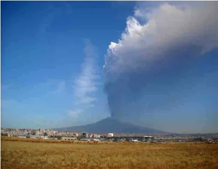
3.4 Etna Ash Cloud 8 September 2011
Following the sunrise on 8 September, Etna produced a series of ash emissions (fig. 2) followed by increased intensity and frequency of the explosions. At about 06:30 GMT, the activity passed from Strombolian into a pulsating lava fountain, accompanied by increasing amounts of volcanic ash. The paroxysm totally ceased around 08:45 GMT.
Figure 2. Eruption of Mount Etna as seen from the airport of Catania; note its height (Etna’s peak is 3350 m high). Photo is
the courtesy of S. Scollo, INGV Catania).
Fig. 3 shows SEVIRI and MODIS data combined into RGB image. The first example is based on 15 min data from MSG2 (fig. 3 above) and the second one on 5 min data from MSG1 (fig. 3 below). The volcanic ash cloud (actually all elevated objects) is coloured because of the wind and the parallax. Sea is white because the colours are inverted (in visible images is sea
normally dark). The yellow part of the cloud corresponds to MODIS data only, cyan to the first SEVIRI image and purple to the second SEVIRI image. The other colours, like dark blue corresponds to the mixture of images – in this case first and second SEVIRI images.
Figure 3. SEVIRI and MODIS data combined into RGB image; above data from 15 min SEVIRI retrieval on MSG2, below data
from 5 min SEVIRI retrieval on MSG1.
The colours make it possible to observe the parallax between MODIS and both SEVIRI images: for the south-eastern “corner” of the cloud we show corresponding points on all three images (fig. 3 above). They are connected with lines corresponding to the parallax between MODIS and first SEVIRI image (parallax 1), MODIS and second SEVIRI Image (parallax 2) and effect of advection between both SEVIRI images (advection).
Figure 4. Cross correlation between MODIS and both SEVIRI images, estimated parallax and corresponding CTH of the ash cloud from Etna; above data from 15 min retrieval from MODIS
and SEVIRI on MSG2, below data from 5 min retrieval from MODIS and SEVIRI on MSG1.
that these results are of lower uncertainty than results based on 15 min data.
4. STEREOSCOPIC OBSERVATIONS FROM A LOW ORBIT
A low orbit (height of 300–500 km) has many advantages over higher orbits when it comes to cloud photogrammetry. Because of its lower height and higher speed, the instruments can reach a suitable baseline between two positions within some seconds. This significantly reduces the influence of wind. In addition, a lower orbit usually means also a higher spatial resolution of data, resulting into higher level of details. This can provide more texture that is necessary for a reliable image matching. Low orbits were not used very often in the past. These orbits have some limitations for other fields of remotes sensing. Its main disadvantage is its narrower swath, which increases also revisit time. Low orbits have gained on importance in the recent years. The reason for that is increased number of launches of small satellites. The philosophy of such satellites is their cost-effectiveness. The most expensive post by a small satellite mission is its launch. As the price of launch depends also on the orbit height, most of small satellites are launched into low orbits.
4.1 Crew Earth Observations
Besides small satellites, into a low orbit was positioned also the International Space Station (ISS). ISS does not carry many sophisticated earth observation instruments. But NASA started some years ago a programme named Crew Earth Observations. Within this programme, the astronauts take photos of the Earth. NASA made available these images for scientific purpose. It is also possible to make an acquisition request of some specific area. The co-author of this paper, Alexander Gerst, was a crew member of ISS missions 40/41. As an acknowledged volcanologist he was asked to provide photos of volcanic clouds. But there was “unfortunately” no major eruption during his mission. He still managed to provide photos of Zhupanovsky volcano (Kamchatka, Russia) during its activity in September 2014 (fig. 5).
Figure 5. A photo (number ISS041e000162) of Zhupanovsky volcano and it ash cloud on Septemebr 10 2014 at 23:11 UTC; it is a courtesy of the Earth Science and Remote Sensing Unit,
NASA Johnson Space Center.
4.2 ISS images pre-processing
Here we have to point out that the used camera contains a typical full-frame sensor. Usual satellite instruments contain a push broom scanner (along track scanner). In a push broom sensor, a line of sensors arranged perpendicular to the flight direction of the spacecraft is used. Different areas of the surface are imaged as the spacecraft flies forward. This means, that each point on earth is scanned only once by such an instrument. But a full frame sensor can take even a video of an area, which is a significant advantage of full-frame sensors over push broom technology.
The main difference between the ISS crew images and data retrieved by classical satellite instruments is that the ISS images are usual photos and not calibrated data. Because the JPG files available in Gateway to Astronaut Photography of Earth (http://eol.jsc.nasa.gov/) contain not enough of radiometric details, especially if a cloud is transparent, we requested RAW files. They contain for each band 14 bit data, which is a huge improvement over 8 bit data given in each JPG channel. We wrote our own code that converts Nikon NEF file to a TIFF file with 16 bit per channel.
Furthermore, the images are not geolocated. In the metadata of each image is given the location of ISS as the image was taken. But to estimate CTH a described by eq. 2 we require also the coordinates of each pixel. An average pixel size in fig. 5 is ~50 m. We have manually georeferenced the image using coastlines and then projected data to UTM projection (zone 57N) in 200 m spatial resolution (fig. 6). It was necessary to choose only points with zero elevation for geolocation, so the higher objects preserved their parallax.
Figure 6. Points (red dots) selected for geolocation of ISS images. Zhupanovsky is in the figure above, in the middle left
you can see also Koryaksky and Avachnisky volcanoes.
For the case study we selected a pair of images ISS041e000162 and ISS041e000164. The time gap between both images was 11.65 s. The ISS moved within this time almost for 130 km. Considering its height was at that time 419 km, the baseline was appropriately long for a reliable image matching at 200 m resolution data. The georeferenced data (only green channel that showed in the case study the largest contrast within the clouds) are shown in fig. 7.
Zhupanovsky volcano
Figure 7. Geolocated green channel of the images numbered ISS041e000162 (left) and ISS041e000164 (right). The red
rectangle shows the extent of results in fig. 8.
We ran basically the same procedure as described in sections 3.2 and 3.3. The position of ISS was retrieved from the web archive http://www.isstracker.com/historical and interpolated to the exact time the image was taken. The relative time between images is given by a hundred of a second. The absolute time accuracy can be as bad as several seconds, because the camera is not synchronized with the GPS. The time on the camera is always set manually. To account for this we have an iterative solution: we change the time of the first image was taken so long that the estimated height of some recognizable mountain peaks agrees with their true elevation.
4.3 Zhupanovsky Ash Cloud 10 September 2014
After 54 years of inactivity, the volcano began erupting on October 23, 2013 and again in 2014, continuing into 2015. Here we present only results for 10 September 2014. For the further processing we decided to focus only on data over sea providing a homogenous background. We have ignored the data in the coastal region because of the turbid water that has approximately the same reflectance as the ash over the sea.
Figure 8. Correlation index over the sea on the left and CTH for pixels that passed the internal accuracy control on the right. The extent of this image is shown with the red rectangle on fig. 7.
The correlation index between both images was very high (fig. 8 left), in most parts of the cloud around 90%, which shows that this procedure is capable of producing good results even over transparent plume. In the end we have filtered out the data having lower correlation, or larger distance between lines of sight and the pixels that remained have height between 7 and 8 km (fig. 8 right). Global Volcanism Program (2014) reported satellite estimation of ash height to be up to 4 km during 9–11 September but it does not provide any source. In this time ash clouds drifted about 1000 km due South.
5. DISCUSSION AND CONCLUSIONS
We presented two innovative ways of CTH estimation. Both use essentially the same methodology but different instruments. The first method has been already validated (Zakšek et al., 2013) – the results for 2010 Eyjafjallajökull eruption had an accuracy of ~600 m. But here we showed that the same methodology can be used also on small clouds that might be still developing. In the case that clouds are still developing in vertical direction, it is obviously better to use SEVIRI data retrieved each 5 min instead of 15 min.
The results based on ISS images have not been validated because we did not have any independent data of this area for the same time. The approximate validation could be possible by comparing the standard MODIS cloud product made on 11 September at 00:45 UTC, but for an accurate comparison is the time gap between ISS and MODI retrieval too large (Terra flew ~90 min later over Zhupanovsky than ISS; see also
http://earthobservatory.nasa.gov/NaturalHazards/view.php?id=8 4386).
For conclusion, we can take a look at advantages and disadvantages of stereoscopic observations more closely. The most important advantage of the proposed method is its independence of physical assumptions. For its use we do not need emissivity of the cloud, it does not matter whether a cloud is close or even above the tropopause, etc. Secondly, the method is perhaps not as fast as CTH estimation from brightness temperature but it is still much faster than some methods depending on the atmospheric transport modelling or radiative transfer modelling. And finally, the method is very accurate, especially if subpixel image matching is applied. An alternative to the image matching is selection of typical points in the ash clouds, like centre of ash mass (personal communication with Stefano Corradini). This procedure has not been practised so far but it is most likely the best option for accurate selection of corresponding points over transparent clouds.
The accuracy of image matching depends mostly on appropriate texture in data. This can be problematic especially with transparent clouds, where the texture of the background becomes dominant. An additional parameter that influences accuracy is the geolocation accuracy of the input images. This should be always (automatically) checked and corrected using independent GIS layers. The greatest issue of the cloud photogrammetry is simultaneous data retrieval from different points. We have here presented only a nearly simultaneous retrieval, but it performed well in both case studies.
ACKNOWLEDGEMENTS
The research has been supported by grants from the German Science Foundation (DFG) number ZA659/1-1.
The SEVIRI L1.5 data were obtained through the online archive of EUMETSAT images (Earth Observation Portal). The MODIS L1B data were obtained through the online Data Pool at the NASA Land Processes Distributed Active Archive Center (LP DAAC), USGS/Earth Resources Observation and Science (EROS) Center, Sioux Falls, South Dakota (https://lpdaac.usgs.gov/get_data). ISS images were obtained through the online Gateway to Astronaut Photography of Earth (http://eol.jsc.nasa.gov/); they are courtesy of the Earth Science and Remote Sensing Unit, NASA Johnson Space Center. The RAW images were provided by ESA and NASA.
REFERENCES
Aksakal, S.K., 2013. Geometric Accuracy Investigations of SEVIRI High Resolution Visible (HRV) Level 1.5 Imagery. Remote Sens. 5, 2475–2491. doi:10.3390/rs5052475
Anderson, C.H., Bergen, J.R., Burt, P.J., Ogden, J.M., 1984. Pyramid Methods in Image Processing. RCA Eng. 29, 33–41.
Bye, B.L., 2010. Volcanic Eruptions: Science And Risk
Management [WWW Document]. URL
http://www.science20.com/planetbye/volcanic_eruptions_scienc e_and_risk_management-79456 (accessed 2.26.13).
Carn, S.A., Pallister, J.S., Lara, L., Ewert, J.W., Watt, S., Prata, A.J., Thomas, R.J., Villarosa, G., 2009. The Unexpected Awakening of Chaitén Volcano, Chile. Eos 90, 205–206. doi:200910.1029/2009EO240001
Chang, F.-L., Minnis, P., Lin, B., Khaiyer, M.M., Palikonda, R., Spangenberg, D.A., 2010. A modified method for inferring upper troposphere cloud top height using the GOES 12 imager 10.7 and 13.3 µm data. J. Geophys. Res. 115, D06208. doi:10.1029/2009JD012304
Dubuisson, P., Frouin, R., Dessailly, D., Duforêt, L., Léon, J.-F., Voss, K., Antoine, D., 2009. Estimating the altitude of aerosol plumes over the ocean from reflectance ratio measurements in the O2 A-band. Remote Sens. Environ. 113, 1899–1911. doi:10.1016/j.rse.2009.04.018
Eckhardt, S., Prata, A.J., Seibert, P., Stebel, K., Stohl, A., 2008. Estimation of the vertical profile of sulfur dioxide injection into the atmosphere by a volcanic eruption using satellite column measurements and inverse transport modeling. Atmospheric Chem. Phys. 8, 3881–3897. doi:10.5194/acp-8-3881-2008
Genkova, I., Seiz, G., Zuidema, P., Zhao, G., Di Girolamo, L., 2007. Cloud top height comparisons from ASTER, MISR, and MODIS for trade wind cumuli. Remote Sens. Environ. 107, 211–222. doi:10.1016/j.rse.2006.07.021
Glaze, L.S., Francis, P.W., Self, S., Rothery, D.A., 1989. The 16 September 1986 eruption of Lascar volcano, north Chile: Satellite investigations. Bull. Volcanol. 51, 149–160. doi:10.1007/BF01067952
Global Volcanism Program, 2014. Zhupanovsky: Weekly
Report [WWW Document]. URL
http://www.volcano.si.edu/volcano.cfm?vn=300120#September 2014
Guffanti, M., Casadevall, T.J., Budding, K., 2010. USGS Data Series 545: Encounters of Aircraft with Volcanic Ash Clouds: A Compilation of Known Incidents, 1953–2009 [WWW Document]. Data Ser. 545. URL http://pubs.usgs.gov/ds/545/ (accessed 2.26.13).
Hasler, A.F., 1981. Stereographic Observations from Geosynchronous Satellites: An Important New Tool for the Atmospheric Sciences. Bull. Am. Meteorol. Soc. 62, 194–212. doi:10.1175/1520-0477(1981)062<0194:SOFGSA>2.0.CO;2
Heinold, B., Tegen, I., Wolke, R., Ansmann, A., Mattis, I., Minikin, A., Schumann, U., Weinzierl, B., 2012. Simulations of the 2010 Eyjafjallajökull volcanic ash dispersal over Europe using COSMO–MUSCAT. Atmos. Environ. 48, 195–204. doi:10.1016/j.atmosenv.2011.05.021
Heymsfield, G.M., Blackmer, R.H., Schotz, S., 1983. Upper-Level Structure of Oklahoma Tornadic Storms on 2 May 1979. I: Radar and Satellite Observations. J. Atmospheric Sci. 40,
1740–1755.
doi:10.1175/1520-0469(1983)040<1740:ULSOOT>2.0.CO;2
Holz, R.E., Ackerman, S.A., Nagle, F.W., Frey, R., Dutcher, S., Kuehn, R.E., Vaughan, M.A., Baum, B., 2008. Global Moderate Resolution Imaging Spectroradiometer (MODIS) cloud detection and height evaluation using CALIOP. J. Geophys. Res. Atmospheres 113, D00A19. doi:10.1029/2008JD009837
Karagulian, F., Clarisse, L., Clerbaux, C., Prata, A.J., Hurtmans, D., Coheur, P.F., 2010. Detection of volcanic SO2, ash, and H2SO4 using the Infrared Atmospheric Sounding Interferometer (IASI). J. Geophys. Res. Atmospheres 115, D00L02. doi:201010.1029/2009JD012786
Kursinski, E.R., Hajj, G.A., Schofield, J.T., Linfield, R.P., Hardy, K.R., 1997. Observing Earth’s atmosphere with radio occultation measurements using the Global Positioning System. J. Geophys. Res. Atmospheres 102, 23429–23465. doi:10.1029/97JD01569
Nelson, D.L., Garay, M.J., Kahn, R.A., Dunst, B.A., 2013. Stereoscopic Height and Wind Retrievals for Aerosol Plumes with the MISR INteractive eXplorer (MINX). Remote Sens. 5, 4593–4628. doi:10.3390/rs5094593
Oppenheimer, C., 1998. Review article: Volcanological applications of meteorological satellites. Int. J. Remote Sens. 19, 2829. doi:10.1080/014311698214307
Prata, A.J., Grant, I.F., 2001. Retrieval of microphysical and morphological properties of volcanic ash plumes from satellite data: Application to Mt Ruapehu, New Zealand. Q. J. R. Meteorol. Soc. 127, 2153–2179. doi:10.1002/qj.49712757615
Prata, A.T., Siems, S.T., Manton, M.J., 2015. Quantification of volcanic cloud-top heights and thicknesses using A-train observations for the 2008 Chaitén eruption. J. Geophys. Res. Atmospheres 2014JD022399. doi:10.1002/2014JD022399
Richards, M., Ackerman, S.A., Pavolonis, M.J., Feltz, W.F., 2006. Volcanic ash cloud heights using the MODIS CO2-slicing algorithm. Presented at the 12th Conference on Aviation Range and Aerospace Meteorology, Atlanata, USA.
Scambos, T.A., Dutkiewicz, M.J., Wilson, J.C., Bindschadler, R.A., 1992. Application of image cross-correlation to the measurement of glacier velocity using satellite image data. Remote Sens. Environ. 42, 177–186. doi:10.1016/0034-4257(92)90101-O
Scollo, S., Kahn, R.A., Nelson, D.L., Coltelli, M., Diner, D.J., Garay, M.J., Realmuto, V.J., 2012. MISR observations of Etna volcanic plumes. J. Geophys. Res. 117, D06210. doi:10.1029/2011JD016625
Solheim, F.S., Vivekanandan, J., Ware, R.H., Rocken, C., 1999. Propagation delays induced in GPS signals by dry air, water vapor, hydrometeors, and other particulates. J. Geophys. Res. Atmospheres 104, 9663–9670. doi:10.1029/1999JD900095
Stohl, A., Prata, A.J., Eckhardt, S., Clarisse, L., Durant, A., Henne, S., Kristiansen, N.I., Minikin, A., Schumann, U., Seibert, P., Stebel, K., Thomas, H.E., Thorsteinsson, T., Tørseth, K., Weinzierl, B., 2011. Determination of time- and height-resolved volcanic ash emissions for quantitative ash dispersion modeling: the 2010 Eyjafjallajökull eruption. Atmospheric Chem. Phys. 11, 5541–5588. doi:10.5194/acpd-11-5541-2011
Tupper, A., Carn, S., Davey, J., Kamada, Y., Potts, R., Prata, F., Tokuno, M., 2004. An evaluation of volcanic cloud detection techniques during recent significant eruptions in the western “Ring of Fire.” Remote Sens. Environ. 91, 27–46. doi:10.1016/j.rse.2004.02.004
Virtanen, T.H., Kolmonen, P., Rodríguez, E., Sogacheva, L., Sundström, A.-M., de Leeuw, G., 2014. Ash plume top height estimation using AATSR. Atmos Meas Tech 7, 2437–2456. doi:10.5194/amt-7-2437-2014
Zakšek, K., Hort, M., Zaletelj, J., Langmann, B., 2013. Monitoring volcanic ash cloud top height through simultaneous retrieval of optical data from polar orbiting and geostationary satellites. Atmospheric Chem. Phys. 13, 2589–2606.