Full Terms & Conditions of access and use can be found at
http://www.tandfonline.com/action/journalInformation?journalCode=ubes20
Download by: [Universitas Maritim Raja Ali Haji] Date: 11 January 2016, At: 22:56
Journal of Business & Economic Statistics
ISSN: 0735-0015 (Print) 1537-2707 (Online) Journal homepage: http://www.tandfonline.com/loi/ubes20
The Distributional Impacts of Minimum Wage
Increases When Both Labor Supply and Labor
Demand Are Endogenous
Tom Ahn, Peter Arcidiacono & Walter Wessels
To cite this article: Tom Ahn, Peter Arcidiacono & Walter Wessels (2011) The Distributional Impacts of Minimum Wage Increases When Both Labor Supply and Labor Demand
Are Endogenous, Journal of Business & Economic Statistics, 29:1, 12-23, DOI: 10.1198/ jbes.2010.07076
To link to this article: http://dx.doi.org/10.1198/jbes.2010.07076
View supplementary material
Published online: 01 Jan 2012.
Submit your article to this journal
Article views: 333
Supplementary materials for this article are available online. Please click the JBES link athttp://pubs.amstat.org.
The Distributional Impacts of Minimum Wage
Increases When Both Labor Supply and
Labor Demand Are Endogenous
Tom A
HNDepartment of Economics, University of Kentucky, Lexington, KY 40506
Peter A
RCIDIACONODepartment of Economics, Duke University, Durham, NC 27708 (psarcidi@econ.duke.edu)
Walter W
ESSELSDepartment of Economics, North Carolina State University, Raleigh, NC 27695
We develop and estimate a one-shot search model with endogenous firm entry, and therefore zero expected profits, and endogenous labor supply. Positive employment effects from a minimum wage increase can result as the employment level depends upon both the numbers of searching firms and workers. Welfare implications are similar to the classical analysis: workers who most want the minimum wage jobs are hurt by the minimum wage hike with workers marginally interested in minimum wage jobs benefiting. We estimate the model using CPS data on teenagers and show that small changes in the employment level are masking large changes in labor supply and demand. Teenagers from well-educated families see increases in their employment probabilities and push out their less-privileged counterparts from the labor market. This article has supplementary material online.
KEY WORDS: Search; Unemployment.
1. INTRODUCTION
Empirical work by Card and Krueger (1994,1995) has called the classical model of the minimum wage as a price floor into question. Their research suggests that an increase in the mini-mum wage may even have small positive employment effects. While there has been considerable controversy regarding their findings (seeNeumark and Wascher 2000and the reply byCard and Krueger 2000) the evidence for strong negative employ-ment effects from an increase in the minimum wage is surpris-ingly weak.
The lack of strong negative employment effects from increas-ing the minimum wage has led some policy makers to support minimum wage increases as a means of transferring money from rich firms to poor workers. In this article we show that changes in the employment level from a minimum wage in-crease may be masking much larger changes in labor supply and labor demand. Further, these larger changes imply employ-ment losses for groups that most wanted the minimum wage jobs in the first place.
In particular, we develop a two-sided search model with en-dogenous labor supply and labor demand that can exhibit pos-itive employment effects from an increase in the minimum wage. In the classical analysis, the number of searching work-ers has no effect on the number of matches. In a more general search model, the number of matches increases with the num-ber of searching workers. Hence, increasing the minimum wage may induce search which can lead to higher employment levels even with the number of firms falling. However, these positive employment effects also lead to lower probabilities of matching at the individual level. As in Luttmer (2007) and Glaeser and
Luttmer (2003), in expectation, those with the lowest reserva-tion wages are hurt most by the increase in the minimum wage. Our search model can therefore generate zero or positive em-ployment effects while also having firms earn zero expected profits both before and after the minimum wage increase. The search model shows that the effect of a minimum wage increase may appear small because the variable used to measure this effect—the employment level—does not adequately capture the churning of the labor market. Individuals induced to enter the labor market result in more matches and may not lower the employment level. However, the new matches push out those who originally wanted minimum wage jobs. Therefore, there are possibly large negative welfare effects from a minimum wage increase, even if the employment level stays constant or increases.
We show that the model developed in the theoretical section is estimable. Estimates of the model yield three sets of parame-ters: (1) the parameters of the wage generating process, (2) the parameters of the firm’s zero profit condition (labor demand), and (3) the parameters of the search decision (labor supply). Although we do not observe firm behavior, we show that the firm’s zero profit condition can be written as a function of the probability of a worker finding a match. The three sets of para-meters can then be estimated from data on wages, employment, and search choices, respectively.
We use a 12-year band (1989 to 2000) of 16 to 19-year-old white teenagers from the basic monthly outgoing rotation CPS
© 2011American Statistical Association Journal of Business & Economic Statistics January 2011, Vol. 29, No. 1 DOI:10.1198/jbes.2010.07076
12
files. We find that the employment elasticity with respect to a minimum wage increase is moderately negative for this group of teenagers. However, this is masking large increases in the probability of search coupled with large decreases in the prob-ability of finding a job conditional on search.
Positive employment effects from a minimum wage in-crease then exist for subgroups of teenagers. In particular, those who come from highly educated families see their employ-ment probabilities increase due to their increased probability of search. In contrast, those who come from less educated families see their employment probabilities fall. These teenagers were more likely to search in the first place and hence the decrease in labor demand outweighs the increase in labor supply. Teenagers from more privileged backgrounds have higher reservation val-ues, but lower search costs as compared to teens from poorer, less-educated families. Raising the minimum wage changes the incentives to entry for these two groups of teens in different ways, with the combination of higher expected wages and lower probabilities of employment being more attractive to the teens from well-educated families. Our results show that a minimum wage hike is then not a transfer from rich firms to poor workers, but frompoorworkers torichworkers. These results are con-sistent with the reduced form results of Lang and Kahn (1998) and Neumark and Wascher (1995) who also show that the ef-fects of minimum wage increases on the composition of the workforce may make raising the minimum wage unattractive. Lang and Kahn find that raising the minimum wage leads to a shift in the fast-food workforce from adults to teenagers, while Neumark and Wascher’s results suggest that minimum wage in-creases lead to a shift in the teenage workforce from those who have completed their schooling to those whose value of school is relatively high.
Estimation of structural search models have a rich history in labor economics (see Eckstein and van den Berg 2007for a review). While there is much variation in the types of search models estimated, all generally rely upon infinitely lived agents in a steady state equilibrium with reservation values determined in part by the continued value of search (see, e.g., Eckstein and Wolpin1990and van den Berg and Ridder1998).
This article builds upon and is most related to Flinn (2002,
2006), which examine the welfare implications of minimum wage increases in a search model where firms and workers split a match-specific output. The main conclusions from Flinn (2006) is that it is possible for a minimum wage increase to be welfare improving, and that modeling assumptions about the endogeneity of contact rates is crucial to the estimation of a welfare maximizing minimum wage. The equivalent of contact rates in our article is the probability of a worker and a firm matching, and we explicitly allow this probability to be endoge-nous. Our model sacrifices the dynamics present in Flinn (2006) in treating search as a one-shot game. However, by making this sacrifice, we are able to develop a richer specification of la-bor supply as well as being able to consider equilibria across states and time. This in turn allows us to examine how mini-mum wages change the composition of the teenage workforce.
The rest of the article proceeds as follows. Section2shows the classical model and how it does and does not relate to the matching model. Section3 develops the two-sided search model, with welfare and employment analysis in Section 4.
Section5describes the data. The translation from the theoreti-cal model to what is estimated is done in Section6. Section7
presents the estimation results. Section 8 performs the policy simulations and Section9concludes.
2. THE CLASSICAL MODEL
The classical analysis of the effects of a minimum wage can be found in most introductory economics textbooks. However, by first examining the classical model it is possible to see why our model is able to generate positive employment effects from an increase in the minimum wage while the classical model is not. Further, the welfare implications of our model will turn out to be very similar to those of the classical model.
Figure1shows the implications of an increase in the mini-mum wage in the classical model. Employment here falls from
Q∗ toQ. Note that the employment level only depends upon labor demand. This is the primary difference between the clas-sical model and matching models. Matching models rely on a “matching function” which takes the number of searching workers and the number of searching firms and produces an em-ployment level. Assuming one vacancy per firm, the matching function in the classical model is the minimum of the number of searching firms and the number of searching workers. The minimum must be the number of searching firms when there is a binding minimum wage. However, other matching functions that depend upon both the number of searching firms and the number of searching workers can produce increases in the em-ployment level because the increased labor supply may more than compensate for the decreased labor demand.
The classical model requires an additional assumption as to how jobs are assigned because there is an excess supply of workers. In Figure 1we have assumed that the probability of employment is the same across searching workers. This proba-bility of finding a minimum wage job would be given byQ/Q
whereQis the number of individuals interested in working at the minimum wage. The area between the labor supply curve and the curve that kinks atQgives the expected output over the reservation wage of the workers. Note that the expected out-put is smaller with the minimum wage increase for all workers belowQc. These are the workers who were most interested in
being employed and would be willing to trade a lower wage for a higher probability of employment.
The matching model described below has very similar wel-fare implications to the classical model. If there are losers be-cause of a minimum wage increase, it will be those individuals who were most interested in being employed. Winners are then those individuals who would either not be interested or only marginally interested in being employed at the market clearing wage.
3. THE MATCHING MODEL
In this section we present a two-sided search model designed to highlight the effects of a minimum wage increase in the low wage market. The model has four components:
1. The decisions by individuals regarding whether to search given their expectations regarding labor market outcomes and their value of leisure.
Figure 1. Classical employment losses from a minimum wage increase.
2. The decisions by firms to search such that, in equilibrium, a zero expected profit decision is satisfied.
3. The process by which workers and firms are paired. 4. The process governing wages.
3.1 Labor Force Participation
There are N individuals available to search and individuals live for one period. Individuals are differentiated in their reser-vation values for not working. Theith individual has reservation value Ri, whereRi is drawn from the cumulative distribution
functionF(R)and has support[0,∞). This reservation value can be leisure or any outside option for the individual. For in-stance, we may assume that Ri is the value of schooling for
teenagers, with the treatment effect of education varying across the population.
Denotepas the probability that a worker matches with a firm conditional on searching, wherepis the same for all individuals in a market. Note that even if an individual does match with a firm, the match may be rejected by either the firm or the worker which will be discussed later in the article. Denote Ki as the
search cost for individuals that is paid whether the searching worker matches with a firm or not.Kiis drawn from the
cumu-lative distribution functionH(K)and has support[K,∞). Individuals are risk neutral with the value of searching (not searching) for individualidenoted byVSi(VNi). The payoff of
matching with a firm is the wage,W, if the wage is above the individual’s reservation value. If the wage is below the indi-vidual’s reservation value, the match will be rejected and the payoff is the reservation value. There is uncertainty with regard to the wage which will be explained later in the article.VSiand VNiare then given by
VSi=pEmax{W,Ri} +(1−pi)Ri−Ki, (1)
VNi=Ri. (2)
Differencing the value of not searching from the value of searching yields the net expected value of searching,Vi, given
by
Vi=pEmax{W−Ri,0} −Ki. (3)
The number of searching workers,N, is endogenous with indi-viduals searching whenVi>0.
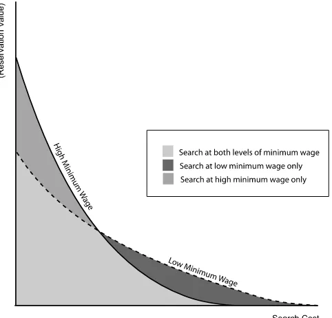
Note that search costs and reservation values affect the deci-sion to search through different channels. See Figure2for an il-lustration. Consider two individuals, one with a high reservation value and a low search cost and another with a low reservation
Figure 2. Effect of reservation values and search costs on search behavior.
value and a high search cost. It is possible to find combinations of wages and probabilities of matching such that the first indi-vidual searches and the other does not. But it is also possible to find wage-probability combinations such that the second indi-vidual searches and the first does not. This case will occur at a higher probability of matching and a lower expected wage: in-dividuals with relatively high search costs and low reservation wages are willing to take lower wages for higher probabilities of matching. The distinction betweenRandK is important, as we show that teens from disadvantaged backgrounds are more likely to have higher search costs and lower reservation wages compared to their more privileged counterparts in the empirical section.
3.2 Firms
The number of firms,J, is endogenous. All firms within a market are identical and therefore have identical probabilities of matching with a worker,q. Production from a match is given by the random variableY, which represents output and firms pay a search cost, C1. Upon matching, the firm may pay an additional cost,C2. (C2turns out to be a negative in most cases.
This parameter may be considered as a partial recoupment of the search cost upon matching.)
We assume that the output of a match is given by
Yij=Y∗exp(ǫij), (4)
whereY∗is the median match value.ǫijis then a match-specific
component with zero median, is drawn from the cumulative dis-tribution functionG(ǫ), and has support(−∞,∞).
Firms enter until all firms have zero expected profits. Ex-pected profits are then given by
qE(max{Yij−Wij,0} −C2)−C1=0, (5)
as firms will reject matches whereYij<Wij.
3.3 Matching
With the search decisions for workers and firms defined above, we now describe how workers are allocated to firms. Workers and firms are matched using a Cobb–Douglas match-ing function with the restriction that the number of matches can be no greater than either the number of searching workers or the number of searching firms. Although many matching functions allow for positive employment effects from an increase in the minimum wage, we use a Cobb–Douglas matching function as in Pissarides (1992) to illustrate the result because of its preva-lence in the literature. (See Petrongolo and Pissarides2001for a review.)
The number of matches is then given by
x=min(AJαN1−α,J,N), (6) whereα∈(0,1)andAis a normalizing constant. All workers and firms within a market have the same probability of finding a match implying thatp=Nx andq=xJ.
3.4 Wages
To close the model, we now specify the wage-generating process. Following Flinn (2006), wages conditional on match-ing followmatch-ing a bargainmatch-ing process where the bargainmatch-ing process produces a spike at the minimum wage. Matched pairs splitYij according to a Rubinstein bargaining game where the
discount factors may vary for the firm and the worker. A suc-cessful match must pay at least the minimum wage,W.
Building on Binmore, Shaked, and Sutton (1989) and Bin-more, Rubinstein, and Wolinsky (1986), we show in the Appen-dix that, under certain assumptions, there is a unique subgame perfect equilibrium of the bargaining game for all matches whereYij≥max{W,Ri}. The unique subgame perfect
equilib-rium outcomes yields the following expression for wages:
Wij=max{βYij,Ri,W}. (7)
β, β ∈(0,1), may be interpreted as the worker’s bargaining strength and represents the difference between the discount fac-tors of the firm and worker. Matches yieldingYij<max{W,Ri}
are unsuccessful. All successful matches where the worker’s share of the revenue would normally be below the minimum wage will earn the same wage even if their match-specific com-ponents differ, thus generating the observed spike at the mini-mum wage. Note that the reservation value does not affect the match revenue division unless the reservation value is higher than both the minimum wage andβ times the revenue of the match.
Proposition1establishes that an equilibrium for this model exists.
Proposition 1. Given Equations (3)–(7), {F(R),G(ǫ),H(K),
C1,C2,α,β,Y∗,W, andN}, there exists an equilibrium inN
andJ.
4. IMPLICATIONS OF THE MODEL
The model described above has a number of implications for a minimum wage increase. In this section we describe how a minimum wage increase affects the probability of matching and conditions under which a minimum wage increase positively affects the employment level. We further show conditions un-der which a minimum wage increases welfare for all searching workers and show which workers are hurt when these condi-tions are not met.
To keep the implications of the model simple, we make an assumption on the primitives to ensure that, in the presence of a minimum wage, any worker who searches will accept any match. Under certain conditions on the primitives, all workers who choose to search for a job will have reservation values less than the minimum wage implying that, Wij =max{βYij,W}.
Namely, suppose the following condition holds:
NR. For allRi>W,
Pr(Yij≥Ri)
E[max{βYij,Ri}|Yij≥Ri] −Ri
−K<0.
Then we are able to establish the following lemma:
Lemma 1. A worker who finds it optimal to search will ac-cept any match.
The expression on the left-hand side of the inequality in
NRrepresents the value of searching given the lowest search cost without the probability of matching. With the probabil-ity of matching ranging between zero and one, only workers who have reservation values below the minimum wage will search whenNRholds. [WhenR>W, individuals search when
pPr(Y≥R)[E(W|Y ≥R)−R] −K>0. The value of p that leads to the highest value of the expression on the left-hand side of the inequality is one. Settingp=1 yields the left-hand side expression inNR.] This is effectively an assumption on the distribution of match revenues,Y, relative to the lowest search cost, K. When the spread of possible revenues is small rela-tive to the search costs, those with reservation values above the minimum wage do not find it worth the risk to search on the off chance that, should they match, the draw on the match revenue will be at least as high as their reservation value.
We next establish that raising the minimum wage will always lower the probability of an individual being employed condi-tional on searching, even if the overall employment level in-creases.
Proposition 2. dWdp <0, regardless of the signs of dWdN, dWdJ, anddWdx.
The intuition comes from examining the expected zero profit condition. An increase in the minimum wage lowers profits conditional on matching, which implies that the probability of matching for the firm must increase for the expected zero profit condition to hold. Since an increase in the probability of match-ing for firms necessarily means a decrease in the probability of matching for workers, we have the result. This holds whether or not the employmentlevelhas increased.
Although the probability of finding a job always falls with an increase in the minimum wage, the effect on the employ-ment level is ambiguous. Proposition3 outlines conditions on the labor demand and supply elasticities under which positive employment effects due to a minimum wage hike are possible.
Proposition 3. dWdx ≥0 ifαεLD+(1−α)εLS≥0, whereεLD
is the elasticity of labor demand andεLSis the elasticity of labor
supply.
Proposition 3 explicitly demonstrates that the direction of growth of employment is jointly dependent on the elasticities of labor supply and demand. Furthermore, since both elastici-ties depend onJandN, which are endogenous, as well asW, the model can exhibit positive or negative employment effects. This is because an increase inW will generally pullJandNin opposite directions, which then leads to labor demand and sup-ply elasticities being pulled in opposite directions. This dual effect on the employment level helps to explain not only why different studies have found positive and negative employment effects, but also why the magnitude of the effects has been so small.
Finally, we show the conditions under which all workers ex-perience a welfare increase from a minimum wage hike. Denote
E1(W)and p1 as the expected wage and probability of
find-ing a match before the minimum wage increase. DenoteE2(W)
andp2as the corresponding values after the minimum wage
in-crease. With reservation values for workers bounded below by
zero, all workers are made better off in expectation by a mini-mum wage increase if
p1E1(W) <p2E2(W).
Establishing when this holds is difficult when matches are re-jected by the firm. That is, whenY<W. However, if we bound the lowest value of productivity at some level Y such that
Y>W, then no matches will be rejected by the firm. With this assumption, we have the following result:
Proposition 4. WhenY>W, all workers benefit from a mar-ginal increase in the minimum wage if and only if 1−α >
E(W) E(Y)−C2.
If firms do reject matches because some match values are below the minimum wage, then the proposition only provides a necessary condition for increasing welfare. This is because raising the minimum wage would lead to more matches being rejected by the firm which is not taken into account in Proposi-tion4.
If the conditions for Proposition 4 are not met, then some workers are made worse off by the increase in the minimum wage. In particular, as discussed in Section 3 and illustrated in Figure2, it is those workers who most want the minimum wage jobs, those with the lowest reservation values, who are hurt by the increase. A minimum wage policy that measures its success by the employment level then misses the important dis-tributional distortion caused by the increase. By increasing the minimum wage, more workers with higher reservation values enter the labor market. While these new workers are undoubt-edly experiencing a welfare increase, workers who were already searching may be worse off, because these are the workers who were most willing to accept a lower paying job for a higher probability of employment.
5. DATA
We now describe the data used in the empirical analysis. We use a 12-year band of the basic monthly outgoing rotation sur-vey files of the Current Population Sursur-vey (CPS) from 1989 to 2000. These 12 years cover four federal minimum wage changes as well as 16 states which changed their state minimum wage to outpace the federal wage. (We exclude Hawaii, Alaska, and District of Columbia from our sample.) Our analysis cov-ers white males who are between 16 and 19 years of age inclu-sive [we ran several specifications, restricting the data to those whose primary residence is with their parent(s) and/or who at-tended school in the last week, with no qualitative differences], using data from nonsummer months (we exclude June, July, and August). From the CPS, we collect hourly wage, whether the individual is searching for work or not, whether the searching worker is employed or not, as well as a number of demographic variables that may affect an individual’s reservation wage and search costs.
Table 1 presents descriptive statistics for three groups of teenagers: the population, job searchers, and those who are em-ployed. Since search is one-shot game, job searchers refer to the sum of those who are unemployed and those who are cur-rently working. Observations with employed individuals earn-ing less than the minimum wage minus 25 cents were dropped,
Table 1. Descriptive statistics
Variable Mean Mean|search Mean|employed
Age 17.48 17.76 17.82
(1.12) (1.08) (1.06)
In school 0.750 0.614 0.613 Head unemployeda 0.060 0.054 0.050 Head othera,b 0.130 0.104 0.097 Head education HS or lessa 0.497 0.493 0.484 Some collegea 0.239 0.263 0.268 College graduatea 0.158 0.154 0.156 Post-collegea 0.106 0.091 0.091 Single parenta 0.297 0.316 0.307 Prime age male unemployment rate 0.036 0.035 0.035
(0.017) (0.017) (0.016)
Pr(search) 0.552
Pr(employed|search) 0.772
Pr(minimum wage binds|employed) 0.167
E(wage|employed) 6.72
(1.74)
Observations 83,478 46,085 35,589
aCalculated only for teenagers identified as living at home and attending school.
bHead other is defined as a household head who cannot be categorized as employed or unemployed.
as well as individuals who reported earning more than $15 per hour (Less that 0.5% of employed workers were cut for making too much, while less than 6% of employed workers were cut for making too little.). As in Flinn (2006), we keep those earn-ing less than a minimum wage but within 25 cents (within 25 cents refers to the nominal wage; after the sample selection, all wages and incomes are adjusted to $2000) because of measure-ment error in reported wages. These observations are treated as earning exactly at the minimum wage. One key variable to the analysis is the prime age male unemployment rate. This unem-ployment rate is calculated at the state-quarter level using CPS data for all males aged 30 to 39. This variable is assumed to affect job search of teenagers only through the expected wage
and the probability of employment, having no effect on search costs or reservation values.
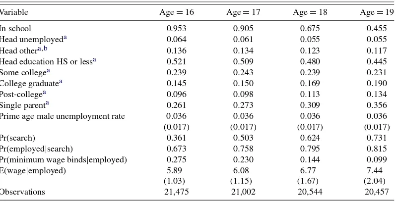
Table1 shows that those who search are more likely to be older and out of school. There is a negative relationship be-tween parental education and the probability of search once we condition on age. Parental characteristics are only calculated for those who are in school and 19 year olds who are in school are more likely to have highly educated parents. This can be seen in Table2which breaks out the descriptive statistics by age.
The descriptive statistics by age show that older teenagers are more likely to participate in the labor market, be out of school, less likely to have their wages bind at the minimum, and have higher expected earnings than their younger
counter-Table 2. Descriptive statistics by age
Variable Age=16 Age=17 Age=18 Age=19 In school 0.953 0.905 0.675 0.455 Head unemployeda 0.064 0.061 0.055 0.055 Head othera,b 0.136 0.134 0.123 0.117 Head education HS or lessa 0.521 0.509 0.480 0.445 Some collegea 0.239 0.243 0.239 0.231 College graduatea 0.145 0.150 0.169 0.190 Post-collegea 0.096 0.098 0.113 0.134 Single parenta 0.261 0.273 0.309 0.356 Prime age male unemployment rate 0.036 0.036 0.036 0.036
(0.017) (0.017) (0.017) (0.017)
Pr(search) 0.361 0.503 0.624 0.731 Pr(employed|search) 0.673 0.758 0.795 0.815 Pr(minimum wage binds|employed) 0.275 0.230 0.144 0.099 E(wage|employed) 5.89 6.08 6.77 7.44
(1.03) (1.15) (1.67) (2.04)
Observations 21,475 21,002 20,544 20,457
aCalculated only for teenagers identified as living at home and attending school.
bHead other is defined as a household head who cannot be categorized as employed or unemployed.
Table 3. State minimum wage from 1989 to 2000
State 1989 1990 1991 1992 1993 1994 1995 1996 1997 1998 1999 2000 California 4.25 4.25 4.25 4.25 4.25 4.25 4.25 4.75 5.15 5.75b 5.75 5.75 Connecticut 4.25 4.25 4.27c 4.27 4.27 4.27 4.27 4.77h 5.18g 5.18 5.65a 6.15a Delaware 3.35 3.80 4.25 4.25 4.25 4.25 4.25 4.75 5.15 5.15 5.65d 5.15h Iowa 3.35 3.85a 4.25a 4.65a 4.65 4.65 4.65 4.75 5.15 5.15 5.15 5.15 Massachusetts 3.75 3.75 3.75 4.25 4.25 4.25 4.25 4.75a 5.25a 5.25 5.25 6.00a Maine 3.75a 3.85a 4.25 4.25 4.25 4.25 4.25 4.75 5.15 5.15 5.15 5.15 Minnesota 3.85a 3.95a 4.25a 4.25 4.25 4.25 4.25 4.75 5.15 5.15 5.15 5.15 New Hampshire 3.65a 3.80 3.85a 4.25c 4.25 4.25 4.25 4.75 5.15 5.15 5.15 5.15 New Jersey 3.35 3.80 3.80 5.05c 5.05 5.05 5.05 5.05 5.15 5.15 5.15 5.15 New York 3.35 3.80 3.80 4.25c 4.25 4.25 4.25 4.75 5.15 5.15 5.15 5.15 Oregon 3.85g 4.25a 4.75a 4.75 4.75 4.75 4.75 4.75 5.50a 6.00a 6.50a 6.50 Pennsylvania 3.70a 3.80 4.25 4.25 4.25 4.25 4.25 4.75 5.15 5.15 5.15 5.15 Rhode Island 4.25f 4.25 4.45c 4.45 4.45 4.45 4.45 4.75 5.15 5.15 5.65e 6.15g Vermont 3.75e 3.85e 4.25 4.25 4.25 4.50a 4.50 4.75 5.25h 5.25 5.75h 5.75 Washington 3.85a 4.25a 4.25 4.25 4.25 4.90a 4.90 4.90 5.15 5.15 5.70a 6.50a Wisconsin 3.65e 3.80 3.80 4.25 4.25 4.25 4.25 4.75 5.15 5.15 5.15 5.15 Other states 3.35 3.80c 4.25c 4.25 4.25 4.25 4.25 4.75h 5.15g 5.15 5.15 5.15
Collected from Nelson (2001). aMinimum wage change on 1/1 or 1/2. bMinimum wage change on 3/1. cMinimum wage change on 4/1. dMinimum wage change on 5/1. eMinimum wage change on 7/1 or 7/2. fMinimum wage change on 8/1. gMinimum wage change on 9/1. hMinimum wage change on 10/1.
parts. Because parental characteristics are calculated only for those identified as attending school, those who have an unem-ployed household head or whose head has low education are more likely to be younger. This is not true for single parent families as divorce is correlated with age of the child.
We use the Monthly Labor Review to collect minimum wage at the state/month level. That is, from 1989 to 2000, we observe the minimum wage in each state, each month. Table3presents the minimum wage in each state, each month within the range of the collected CPS data. These minimum wages are nominal values. In the analysis, the wages and incomes are inflated to $2000.
6. PARAMETERIZING THE MODEL
In this section we show how to estimate the structural model. Estimation has three components. First, for those individuals who successfully match we observe wages. Second, we need to estimate the parameters of the zero profit condition. Although we do not observe the probability of a firm finding a match, we are able to rewrite the zero profit condition as a function of the individual’s probability of finding a match. Finally, we observe decisions by individuals as to whether to search. We can use these decisions to estimate the supply side parameters. In practice, we estimate the model in two stages, first estimating the wage parameters and the zero profit parameters and then estimating the worker search parameters in a second stage.
6.1 Parameterizing Wages
Before specifying the distribution of wages, we first must specify the source of the wages: the output of the match,Yij.
We assume thatYijis given by
Yij=exp(Xiθ )·exp(ǫij), (8)
whereXi are characteristics of individuali’s market (a market
is defined at the age, state, quarter, year level) andθis the set of parameters to be estimated. Because the left tail of the wage distribution is so important to this analysis, we do not make the standard assumption of log-normality on theǫ’s. Rather, we mix over two log-normal distributions allowing both the means and the variances of these distributions to vary. The probability of a draw coming from therth distribution is then given byπr
where therth distribution is distributed N(μr, σr). In addition,
we allow the variance terms to differ by age, definingσ2∗ as
σrk2∗=σr2·Ak, whereAk is an age-specific constant. (We set A16=1, and estimateA17,A18, andA19.)
We assume that condition NR holds implying that only firms reject matches in the presence of a binding minimum wage. That is, if a teenager finds it optimal to search, he is will-ing to accept a minimum wage job. We estimated reduced-form wage equations to see if the factors that influenced the reservations values (e.g., parental education) also influenced the wage. We found no evidence that higher (lower) reservation val-ues were associated with higher (lower) wages. We also tested whether minimum wages had spillover effects by including a dummy variable for whether the minimum wage had been in-creased in the month prior. If spillovers exist, then we would
expect a positive effect on log wages outside of the spike at the minimum wage. We found no evidence of spillover effects. With this condition, the wage generating process is given by
Wij =min{βYij,W}, implying that when the minimum wage
does not bind log wages are given by
ln(Wij)=Xiθ+ln(β)+ǫij. (9)
In the presence of a minimum wage the wage distribution is then distributed truncated log-normal with censoring at the min-imum wage. The truncation occurs when the match value is so low that the firm rejects the match. This occurs whenever
W>Yij. There are then three relevant regions for the quality of
the match:
βYij>W ⇒ {Wij=βYij},
Yij≥W> βYij ⇒ {Wij=W},
W>Yij ⇒ {No match}.
We then observe successful matches for those who are em-ployed at or above the minimum wage.
LetN11andN12indicate the number of individuals who have
wage observations above and at the minimum wage, respec-tively. Defining andφ as the cdfs and pdfs of the standard normal distribution, the likelihood for these observations then follows:
The likelihood above is conditional on the firm not rejecting the match. The denominator in both expressions is one minus the probability that the revenue of the match is so low that the firm would rather not match than pay the minimum wage. The first expression then gives the conditional likelihood of wages above the minimum wage while the second expression is the conditional likelihood of receiving exactly the minimum wage. Note here thatσrk∗ is age specific for the observed teenager.
6.2 Parameterizing Firms
Although we have no information on the firm, we can infer the parameters of the profit function by rewriting the zero profit condition as a function of the individual’s probability of finding a match. To see this, note that the probability of finding a match for firms and workers is given by
q=A
Substituting forqas a function ofpin the zero expected profit condition and solving forpyields
p=δE(max{Y−W,0} −C2)(α)/(1−α), (10)
where
δ=C1−α/(1−α)A−1/(1−α).
This zero expected profit condition is satisfied for every econ-omy. That is, zero expected profits hold by age, state, quarter, and year.
Given the assumed log-normal distribution of Y and the parameters of the wage-generating process, we can calculate
E(max{Y−W,0}), the expected surplus from matching. This surplus can be broken down into three parts: (1) when the match value is high enough such that the minimum wage does not bind, Y˜1, (2) when the match value is such that the minimum wage binds,Y˜2, and (3) when the match value is so low that the firm rejects the match. The last of these parts,Y˜3yields an
ex-pected revenue of zero. Since we estimate the wage distribution assuming all matches are successful, we have a natural test of this assumption from the zero expected profit function. In par-ticular, we test whether the bargaining parameter is low enough such that this region has no observations.Y˜1andY˜2are given
by
We then defineY˜ such that
˜
Y=E(max{Y−W,0})= ˜Y1+ ˜Y2 (11)
implying that the probability of a working matching with a firm can be written as
p=δ(Y˜−C2)α/(1−α). (12)
Here we can see the advantage of the additional parameter,C2.
Namely, ifαis 0.5, thenδC2serves as an intercept term with the
slope given byδitself. The model fit is substantially improved by adding this term.
However, in the data we do not observe whether an individual is matched with a firm,p, but only observeptimes the proba-bility that the match is successful,pψ, whereψis given by
ψ=1−
lnW−Xθ
σrk∗
.
Positive search outcomes for workers are then Bernoulli draws frompψ. The likelihood function is then given by
L2=
whereN2is the number of searching workers andmi indicates
whether or not theith worker was matched. We allow theδ’s andC2’s to vary by state.
6.3 Parameterizing the Individual
We now turn to the decision by individuals as to whether or not to search. Recall that an individual searches if
pψ (E(W)−Ri)−Ki>0.
Because pψ is multiplicatively attached to Ri, but not to Ki,
even if the observed variables are common acrossRi andKi,
we can separately identify their coefficients. With the estimates from the previous two stages it is possible to calculate expected wages and the probability of employment for each individual.
We parameterizeRiandKisuch that all workers have positive
reservation values and search costs
Ri=exp(Z1iγ1+ηi), Ki=exp(Z2iγ2).
Ziis then a vector of demographic characteristics which affect
the individual’s outside option, the γ1’s are the coefficients to
be estimated, andηiis the unobserved portion of the reservation
value.
Family background characteristics are allowed to operate through both the search costs and the reservations values while we include state, year, and quarter fixed effects only in the reser-vation values.
Individuals who come from privileged backgrounds may have high reservation values, making search less likely. How-ever, these same individuals may also have lower search costs. What separately identifies search costs from reservation values is how individuals react to the probability of finding a job. In particular, those with low search costs but high reservation val-ues will be more willing to trade off higher expected wages con-ditional on matching for lower probabilities of employment. In contrast, those with high search costs but low reservation values prefer lower wages coupled with higher match probabilities.
We allow the unobserved portion of the reservation value to be drawn from two different logistic distributions, one for teens who are attending school (l=1) and another for teens who are not attending (l=0). Substituting in and solving forηil shows
that an individual will search when
ηil<ln
We assume that theηl’s are logistically distributed with mean
zero and varianceσl2. Since we do not observe theη’s, the like-lihood function is given by
L3=
tential searchers, andsiis an indicator for whether theith
indi-vidual chose to search. In the standard logit, all coefficients are relative to the variance term. Here we can actually estimateσl
as there is no other natural interpretation for the coefficient on the expression inside the log. Theγ∗’s are then theγ’s divided by the variance scale parameter,σl.
7. RESULTS
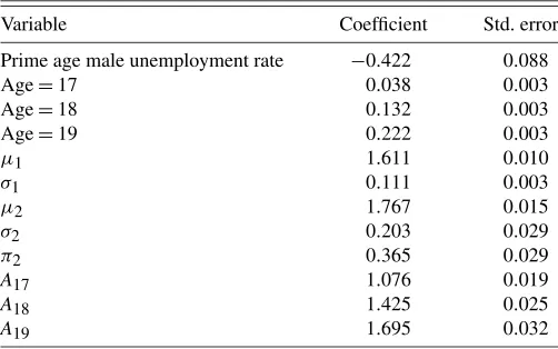
Having specified the estimation strategy, we now turn to the results. The estimates of the wage generating process are given in Table4. In addition to the reported parameters, we also in-cluded state, year, and quarter fixed effects. The coefficient on the prime age male unemployment rate is negative and signifi-cant. This will be important for the analysis of searching as this is our exclusion restriction: the adult unemployment rate only affects search through the expected wage and the probability of finding a match. Mixing over two log-normals shows that higher log wages are associated with higher variances. Vari-ances on unobserved match-specific component increase with age, suggesting that having a common variance term would under-predict the fraction of 19 year olds at the minimum wage while over-predicting the fraction of 16 year olds at the mini-mum.
Estimates of the zero profit condition parameters are given in Table 5. These are β, the bargaining parameter, α, which measures how sensitive the number of matches are relative to the number of searching firms, a conglomerate parameter,δ,
Table 4. Parameters of the wage generating processa
Variable Coefficient Std. error Prime age male unemployment rate −0.422 0.088
Age=17 0.038 0.003
aEstimated jointly with the parameters of the zero condition given in Table5. Estima-tion also included state, year, and quarter fixed effects.
Table 5. Estimates of the firm’s zero profit conditiona
aEstimated on 46,080 white male teenagers who were either employed or looking for a job. Average values forC−1α/(1−α)A−1andC2, which were calculated for each state, are presented.
which is a function of the search cost (C1) and the efficiency of
the matching function, andC2, the recoupment cost. Note that δ andC2 are allowed to vary by state. The relative weight of
firms to workers in determining the probability of matching,α, is estimated at close to 0.45—a result that is in line the macro-economics literature (Peterongolo and Pissarides2001). The es-timatedβis around 0.34, which is similar to the estimates from Flinn (2006).
With the estimates of the log wage regression and the para-meters of the zero-profit condition, we calculate the probability of matching and the expected wages conditional on matching. We then use these estimates to estimate the value of search with the results presented in Table6. The last two numbers in the table give 1/σ for those who are in school and those who are out of school. These numbers are crucial in estimating the wage elasticity. If the numbers are small, participation is driven pri-marily by unobserved reservation values. High values, in con-trast, mean that individuals are very responsive to conditions in the labor market. The parameter estimates imply a labor sup-ply elasticity of 2.48 for those who are in school with a corre-sponding labor supply elasticity of 0.75 for those who are out of school. The large gap in labor supply elasticities is driven part by the fact that the base level of labor force participation
Table 6. Estimates of the search parametersa
Reservation Search
Variable values costs
In school
Household head unemployed −0.026 0.125
(0.086) (0.062)
Household head post-college 1.473 −4.672
(0.109) (3.145)
aEstimated on 83,478 white male teenagers. Estimation of reservation values also in-cluded age, state, year, and quarter fixed effects.
bSearch costs are constant for teens out of school.
is actually quite high for those who are not in school. Note that these calculations hold the probability of finding employment fixed, which will not be the case when we simulate the effects of a minimum wage increase.
Reservation values and search costs are also reported in Ta-ble6. In virtually all cases, a characteristic that leads to a higher reservation value also leads to a lower search cost. This makes sense. Those who have access to technologies that might lower search costs (computers, contacts, etc.) also are likely to be pro-vided with more income from their parents, leading to higher reservation values. Higher parental education and coming from a two-parent family is then associated with lower search costs and higher reservation values. More advantaged backgrounds are then associated with individuals who are more likely to be willing to trade a lower probability of finding a job for a higher wage conditional on employment.
8. ELASTICITIES
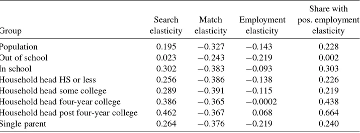
With the estimates of the model in hand, we now see how the minimum wage affects the probability of search, the probabil-ity of obtaining employment conditional on search, and the un-conditional probability of employment. The elasticities of these three variables with respect to increasing the minimum wage are given in the first three columns of Table7.
The table shows that with a minimum wage increase the probability of searching increases. However, this is counter-acted by a decrease in the probability of finding a job condi-tional on searching leading to an overall employment elastic-ity of−0.143. This overall employment elasticity is masking much large changes in labor supply and demand. Namely, the search elasticity with respect to the minimum wage is 0.195 while the match elasticity, how the probability of employment conditional on search changes with an increase in the minimum wage, is−0.327. Therefore, while there is a large decrease in the probability of employment conditional on searching, the overall employment elasticity is buoyed by the increase in the number of searching workers.
The changes in employment and search are not uniform across the population. The next two rows show that the search elasticities are much higher for those who are in school than those who are out of school. These differences in search elastic-ities then lead to overall employment elasticelastic-ities that are twice as large for those out of school than those in school. Hence, there is a shift in the composition of employment away from those who are out of school and towards those who are in school.
Compositional effects are also important within the in-school population. Namely, higher search elasticities are seen for those with two-parent families with highly educated parents. Indeed, those who have a household head with more than a college degree have such large search elasticities that the overall em-ployment effect for this group is positive. This is driven by the positive search elasticities for this group being 1.8 times larger than those whose who have a household head who dropped out before completing high school. These individuals are more re-sponsive to the increase in the minimum wage, in part because they were less likely to search in the first place but also because
Table 7. Minimum wage elasticities
Share with Search Match Employment pos. employment Group elasticity elasticity elasticity elasticity Population 0.195 −0.327 −0.143 0.228 Out of school 0.023 −0.243 −0.219 0.002 In school 0.302 −0.383 −0.093 0.303 Household head HS or less 0.256 −0.386 −0.138 0.226 Household head some college 0.289 −0.391 −0.115 0.219 Household head four-year college 0.386 −0.365 −0.0002 0.438 Household head post four-year college 0.462 −0.367 0.068 0.664 Single parent 0.264 −0.376 −0.219 0.240
these individuals are more willing to trade off a lower probabil-ity of employment for a higher expected wage conditional on employment.
The fourth column shows the share of individuals in partic-ular groups who see their expected probability of employment increase with an increase in the minimum wage. Although al-most 23% see their probability of employment increase, these are confined strictly to those who are in school. For those who are in school, we see that those with the most educated parents are three times as likely to experience a positive employment effect in expectation than those who have the least educated parents. Note that any increase in the probability of employ-ment is being driven by the increased probability of searching as the probability of finding employment conditional on search-ing always falls with an increase in the minimum wage.
Although our methodologies are very different, these results echo the concerns raised by Lang and Kahn (1998) and Neu-mark and Wascher (1994) on the composition effects of mini-mum wage increases. We see an employment shift from those teenagers who are out of school to teenagers who are in school. For those who are in school, there is an employment shift from those who come from single-parent families where the parent has little education to two parent families where the household head is highly educated.
9. CONCLUSION
This article has developed two-sided matching model to ex-plain the puzzling absence of a large impact on employment levels when the minimum wage is increased. In the classical framework, the exit by firms would dictate a decrease in em-ployment. However, more general matching functions can gen-erate positive employment effects from an increase in the min-imum wage. In particular, if employment depends upon both
the number of searching workers and the number of search-ing firms, the increase in the number of searchsearch-ing workers may more than offset the decrease in the number of searching firms. Even if positive employment effects result from a minimum wage hike, however, the probability of any individual worker finding a job has fallen. With employment probabilities falling, if any individuals are hurt from the minimum wage hike it will be those individuals who want the minimum wage jobs the most.
Estimating the structural model was made feasible by trans-lating the firm’s zero profit condition into a function of the
probability of a searching worker finding a match. The esti-mates of the model allow us to decompose the employment effects into their labor supply and labor demand components. Consistent with the theory, we find small employment effects that are masking much larger changes in labor supply and labor demand.
While the employment effects are muted in the population of teenagers we considered, there are large disparities for certain subgroups. Increases in the minimum wage lead to a shift from teenagers who are out school to teenagers who are in school. Further, those teenagers who are in school and have highly ed-ucated parents are likely to see positive employment effects as a result of their increased probability of search. In contrast, those who have less educated parents and/or come from single-parent households see their employment probabilities fall. The overall composition of the low-wage workforce then shifts away from those with disadvantaged backgrounds.
While this study has focused on teenagers, the potential ef-fects of these teenagers on the market for adults in the low-wage labor market are large. The small employment effects found in the previous literature may be masking much larger effects for those adults who find themselves in the low-wage labor mar-ket. This group is likely to be searching for work regardless of the minimum wage and may be pushed out of the labor market by teenagers induced to search because of the higher minimum wage.
SUPPLEMENTAL MATERIALS
Proofs: Supplemental Appendix with proofs. It can also be
downloaded from www.econ.duke.edu/~psarcidi/Appendix forJBES.pdf. (AppendixforJBES.pdf)
ACKNOWLEDGMENTS
We thank Pat Bayer, Chris Flinn, John Kennan, Michael Pries, Curtis Taylor, and seminar participants at Duke Univer-sity, Penn State UniverUniver-sity, New York UniverUniver-sity, University of Maryland, University of Minnesota, Heinz School, Notre Dame, Texas A&M, University of Wisconsin, Yale University, and the 2004 SEA Meetings.
[Received April 2007. Revised December 2008.]
REFERENCES
Binmore, K., Rubinstein, A., and Wolinsky, A. (1986), “The Nash Bargaining Solution in Economic Bargaining,”RAND Journal of Economics, 17, 176– 188. [15]
Binmore, K., Shaked, A., and Sutton, J. (1989), “An Outside Option Experi-ment,”Quarterly Journal of Economics, 104 (4), 753–770. [15]
Card, D., and Krueger, A. B. (1994), “Minimum Wage and Employment: A Case Study of the Fast-Food Industry in New Jersey and Pennsylvania,”
American Economic Review, 84, 772–793. [12]
(1995),Myth and Measurement: The New Economics of the Minimum Wage, Princeton, NJ: Princeton University Press. [12]
(2000), “Minimum Wages and Employment: A Case Study of the Fast-Food Industry in New Jersey and Pennsylvania: Reply,”American Eco-nomic Review, 90 (5), 1397–1420. [12]
Eckstein, Z., and van den Berg, G. J. (2007), “Empirical Labor Search: A Sur-vey,”Journal of Econometrics, 136 (2), 531–564. [13]
Eckstein, Z., and Wolpin, K. I. (1990), “Estimating a Market Equilibrium Search Model From Panel Data on Individuals,”Econometrica, 58, 783– 808. [13]
Flinn, C. (2002), “Interpreting Minimum Wage Effects on Wage Distributions: A Cautionary Tale,”Annales d’Économie et de Statistique, 67–68, 309–355. [13]
(2006), “Minimum Wage Effects on Labor Market Outcomes Un-der Search, Matching, and Endogenous Contact Rates,”Econometrica, 74, 571–627. [13,15,17,21]
Glaeser, E., and Luttmer, E. (2003), “The Misallocation of Housing Under Rent Control,”American Economic Review, 93 (4), 1027–1046. [12]
Lang, K., and Kahn, S. (1998), “The Effect of Minimum-Wage Laws on the Distribution of Employment: Theory and Evidence,”Journal of Public Eco-nomics, 69 (1), 67–82. [13,22]
Luttmer, E. (2007), “Does the Minimum Wage Cause Inefficient Rationing?”
The B.E. Journal of Economic Analysis & Policy, 7 (1) (Contributions), Article 49. [12]
Nelson, R. (2001), “State Labor Legislation Enacted in 2000,”Monthly Labor Review, 124, 12–24. [18]
Neumark, D., and Wascher, W. (1994), “Employment Effect of Minimum and Subminimum Wages: Reply to Card, Katz and Krueger,”Industrial and La-bor Relations Review, 47, 497–512. [22]
(1995), “Minimum Wage Effects on Employment and School Enroll-ment,”Journal of Business & Economic Statistics, 13 (2), 199–206. [13]
(2000), “Minimum Wages and Employment: A Case Study of the Fast-Food Industry in New Jersey and Pennsylvania: Comment,”American Economic Review, 90 (5), 1362–1396. [12]
Petrongolo, B., and Pissarides, C. (2001), “Looking Into the Black Box: A Sur-vey of the Matching Function,”Journal of Economic Literature, 39 (2), 390–431. [15,21]
Pissarides, C. (1992), “Loss of Skill During Unemployment and the Persistence of Employment Shocks,”Quarterly Journal of Economics, 107 (4), 1371– 1391. [15]
van den Berg, G. J., and Ridder, G. (1998), “An Empirical Equilibrium Search Model of the Labor Market,”Econometrica, 66, 1183–1221. [13]