Full Terms & Conditions of access and use can be found at
http://www.tandfonline.com/action/journalInformation?journalCode=ubes20
Download by: [Universitas Maritim Raja Ali Haji] Date: 11 January 2016, At: 23:11
Journal of Business & Economic Statistics
ISSN: 0735-0015 (Print) 1537-2707 (Online) Journal homepage: http://www.tandfonline.com/loi/ubes20
Volatility Jumps
Viktor Todorov & George Tauchen
To cite this article: Viktor Todorov & George Tauchen (2011) Volatility Jumps, Journal of
Business & Economic Statistics, 29:3, 356-371, DOI: 10.1198/jbes.2010.08342
To link to this article: http://dx.doi.org/10.1198/jbes.2010.08342
Published online: 01 Jan 2012.
Submit your article to this journal
Article views: 359
View related articles
Volatility Jumps
Viktor T
ODOROVDepartment of Finance, Kellogg School of Management, Northwestern University, Evanston, IL 60208 (v-todorov@kellogg.northwestern.edu)
George T
AUCHENDepartment of Economics, Duke University, Durham, NC 27708 (george.tauchen@duke.edu)
The article undertakes a nonparametric analysis of the high-frequency movements in stock market volatil-ity using very finely sampled data on the VIX volatilvolatil-ity index compiled from options data by the CBOE. We derive theoretically the link between pathwise properties of the latent spot volatility and the VIX in-dex, such as presence of continuous martingale and/or jumps, and further show how to make statistical inference about them from the observed data. Our empirical results suggest that volatility is a pure jump process with jumps of infinite variation and activity close to that of a continuous martingale. Additional empirical work shows that jumps in volatility and price level in most cases occur together, are strongly dependent, and have opposite sign. The latter suggests that jumps are an important channel for generating leverage effect.
KEY WORDS: Activity index; Jump risk premium; Leverage effect; Stochastic volatility; VIX index.
1. INTRODUCTION
Jumps are intrinsically a continuous time concept that can be defined only relative to a theoretical stochastic process sat-isfying mild regularity conditions. Models for such processes are convenient paradigms that should, of course, provide close approximations to the dynamics of discretely observed data. Models without jumps, that is, models with continuous sam-ple paths, are especially convenient because then asset prices respond in a locally linear manner, hedging arguments work, and convenient, easy to manipulate closed-form expressions for the reduced forms of economic models are available. In the presence of jumps, however, markets are fundamentally incomplete and the analysis far less tractable. A fairly com-plete discussions of the complications induced by jumps is Cont and Tankov (2004), chapter 10, pp. 319–351. Technical issues aside, jumps are important because they represent a signifi-cant source of non-diversifiable risk as discussed at length in Bollerslev, Law, and Tauchen(2008) and the references therein. Policy makers must make decisions in real time during times of jump-inducing chaotic conditions in financial markets, and it is thereby economically important to develop a statistical under-standing of the time series behavior of jumps.
There is currently fairly compelling empirical evidence for jumps in the level of financial prices. The most convincing evidence comes from recent nonparametric work using high-frequency data as in Barndorff-Nielsen and Shephard (2007) and Ait-Sahalia and Jacod (2009a) among others. Preceding that evidence are the findings from parametric studies using daily data such as Chernov et al.(2003),Andersen, Benzoni, and Lund (2002), and Eraker, Johannes, and Polson (2003), which are strongly suggestive but arguably not overwhelming evidence for price jumps in the daily record.
A very prominent model that underlies much empirical work for continuous time processes with jumps is the setup ofDuffie, Pan, and Singleton(2000), which we call here theaffine double-jump model. Since the double-jump model is in the affine class, just as inHeston(1993), it admits reduced form solutions for as-set prices and derivatives that are closed form in the sense that
they can be readily computed on modern computing equipment using straightforward numerical techniques for Fourier series and ordinary differential equations. The double-jump model presumes rare jumps, for example, compound Poisson process, for both asset prices and their variances. It has been applied em-pirically byBroadie, Chernov, and Johannes(2007),Chernov et al.(2003),Eraker, Johannes, and Polson(2003), andEraker (2004) among others (see also empirical work byWu 2010who allows for the jumps to be of infinite activity). It is especially useful for specification and estimation of continuous time mod-els that use data on both the underlying security and deriva-tives written on it. These studies generally find evidence for both jumps in the price level and its volatility.
In this article we aim to understand better the nature of changes, both small and big, in the market volatility, which have important implications for volatility modeling, develop-ing hedgdevelop-ing strategies and specification of market risk premia. In particular we answer the following questions. Is the market volatility moving through occasional and relatively infrequent changes like in a model driven by a compound Poisson process, or it involves a lot of small moves, which over short intervals look like Gaussian as in theHeston(1993) model? Are there “sufficiently big” moves in the volatility to justify inclusion of jumps in its modeling? Are volatility and price jumps related?
To date, the answers to these questions come predominantly through estimation of parametric models built around the affine double-jump model (the recent nonparametric results ofBandi and Reno 2008,2009are an exception). However, these ques-tions are intrinsically nonparametric and importantly they are related with the properties of the observed paths of the volatil-ity for which we do not need long-span asymptotics. Therefore, the persistence in volatility, for example, how many autore-gressive factors are needed for its modeling, is a completely
© 2011American Statistical Association Journal of Business & Economic Statistics July 2011, Vol. 29, No. 3 DOI:10.1198/jbes.2010.08342
356
separate issue from the type of changes through which the volatility evolves over time. Here we are interested in the lat-ter. Goodness-of-fit type tests for parametric volatility models would inevitably be joint type hypothesis and therefore they should always be interpreted with caution when making con-clusions about pathwise properties of volatility. Here, we sepa-rate the pathwise properties of volatility from its long-span ones (like persistence) by using high-frequency data and resorting to fill-in asymptotics. The analysis is fully nonparametric and thus the evidence we provide here is robust.
Our estimation is based on inferring from the data the value of a generalized activity index (Ait-Sahalia and Jacod 2009a and Todorov and Tauchen 2010a), which is a generalization of the classical Blumenthal–Getoor index ofBlumenthal and Getoor(1961). The generalized activity index is defined for an arbitrary stochastic process unlike the Blumenthal–Getoor in-dex which is defined for jump processes only. It lies in the inter-val[0,2]and measures the vibrancy of the process. The index divides the stochastic processes used in the volatility modeling into equivalence classes. For example, the compound Poisson jump process, which is a building block in the affine double-jump model has an activity level of 0. On the other extreme is the Brownian motion (and any diffusion process), whose ac-tivity is 2. Values of the index in (0,1)correspond to jump processes of finite variation, that is, processes whose trajecto-ries over finite intervals are finite. Values of the index in(1,2) correspond to jump processes of infinite variation, that is, their trajectories over finite intervals have infinite length.
We estimate the activity index of high-frequency data on the VIX volatility index computed by the Chicago Board of Op-tions Exchange (CBOE), which is based on close-to-maturity S&P 500 index options, and then make inferences about activ-ity level of the unobserved market volatilactiv-ity. Our estimation of the activity is based on constructing from the high-frequency data an activity signature function, a diagnostic tool proposed inTodorov and Tauchen(2010a). The latter provides also evi-dence whether the “big” moves in volatility should be modeled as jumps. Finally, to explore the link between the discontinu-ities on market level and market volatility we use cojumping statistics proposed inJacod and Todorov(2009).
The nonparametric evidence regarding the types of moves in the market volatility provides empirical information on the plausibility of the various parametric volatility models that have been proposed in the literature. The set of parametric models includes the double-jump model discussed above along with many others reviewed in Section 3 below. In some of these models volatility is continuous, and in others it is a pure jump process. Of course there are also models with both continuous and jump components. The various parametric models have dif-ferent implications for the activity level of the VIX index, the presence of jumps in it and their relationship with the ones in the price level. We find that our nonparametric evidence identi-fies with reasonable accuracy the most plausible class of para-metric models and rules out many others.
There are certain advantages and also some notable pit-falls entailed with using the VIX data. High-frequency data, of course, provide far more information about jumps, both large and small, than do daily data, which is a major plus. Further-more, since the VIX index is computed from quoted options
prices, which are highly sensitive to volatility, it provides far more information on volatility than does the financial price se-ries itself. Some care is needed, however, because the VIX in-dex is not a direct measure of volatility, but rather it is actually the forward price, and thus a risk-neutral expectation, of future variance. The issues are discussed in more detail below. Finally, volatility is known to be a long memory process, and this inter-acts with the VIX index in some subtle ways regarding traded securities, semimartingales, and lack of arbitrage. As discussed below, it turns out that use of the general activity index permits us to separate jumps from long memory, and therefore we can make statements about the characteristics of volatility jumps without having to account for the long memory.
Turning to our main empirical findings, we can summarize them as follows. First, we find that market volatility is a very vibrant process—it involves many small changes as well as oc-casional big moves. The presence of big moves justifies the use of jumps in volatility modeling. In terms of modeling the small moves in volatility we find some evidence against using Brown-ian motion because it is somewhat more “active” than what the data implies for the volatility. On the other hand, the “activity” of the small volatility changes cannot be captured by a com-pound Poisson process or even a process of finite variation like a Lévy subordinator (i.e., a jump process with nonnegative incre-ments as in the non-Gaussian OU model ofBarndorff-Nielsen and Shephard 2001). The reason for this is that a finite variation jump process would imply too “little” activity in volatility than what is observed. We conclude that a model for the volatility that can reconcile the empirical evidence is a pure jump model, where the driving jump process is far more active than a process of finite variation, but on the other hand not as active as a con-tinuous martingale (though the jump activity that we estimate from the data is nevertheless relatively close to that of a con-tinuous martingale). This is to be contrasted with our findings about the market level where we find that we need a continuous martingale to capture the small changes and jumps to capture the big ones.
Second, using both high-frequency data on the VIX index as well as the S&P 500 index, we find strong evidence that the jumps in the volatility and the price level occur at the same time. We also find that these jumps exhibit strong negative depen-dence. These findings suggest that the underlying risks behind the occurrence of stock market discontinuities and the spikes in market volatility (and the corresponding risk premia) are simi-lar if not the same. Therefore plausible equilibrium-based mod-els for the market risk premia should be able to generate en-dogenously such links between volatility and jump risk (and their compensation).
The article is organized as follows. In Section2we define the measures of stochastic volatility and in particular the VIX in-dex, data on which is used in the empirical part. In Section3we present some popular stochastic volatility models and analyze their implications for the VIX index. Section4introduces our measure of activity of a continuous-time process and proposes methods for its inference from discrete observations. Section5 applies the estimation technique to simulated data and Section6 contains the empirical part. Finally Section7concludes.
2. THE VIX INDEX
Let{St}t≥0denote the log of a financial price evolving in
con-tinuous time. We are interested in the high frequency dynamics of the so-called volatility index (VIX) pertaining toSt. The VIX index is computed by the CBOE for the S&P 500 index using written options on it, but the methodology for its computation can be applied to other assets as well. Theoretically, the VIX in-dex is based on a portfolio of out-of-the-money options written onStover a continuum of strike prices whose value equals that of a variance swap; see, for example,Britten-Jones and Neu-berger(2000),Jiang and Tian(2005), andCarr and Wu(2009). The latter is defined as a forward contract on the total quadratic variation of the log-price of the underlying asset over a fixed interval into the future. Following Protter (2004), pp. 66–76, let
[S,S]denote the quadratic variation process associated withSt. Hence the VIX index is given by
vt≡EQ([S,S]t+N− [S,S]t|Ft), (2.1) where N >0 is fixed, {Ft} is the filtration on the
probabil-ity space on which {St}t≥0 is defined, and the expectation is
taken under the risk-neutral distributionQ. Note that in prac-tice the volatility index is typically quoted in terms of annual-ized volatility, which is easier to interpret, but the form (2.1) is much simpler to work with theoretically so we stick with that. The quadratic variation process[S,S]is adapted, increas-ing, càdlàg (i.e., with paths that are a.s. right continuous with left limits), and it can be split into continuous and discontinu-ous components
[S,S]t= [S,S]ct + [S,S]dt, (2.2) corresponding, respectively, to the quadratic variation of the continuous and discontinuous parts of the price processSt. We make a standard assumption in finance and impose absolute continuity of[S,S]ct, that is, stantaneous variance byAndersen et al.(2009). The spot vari-ance σt2 is the instantaneous increment to the quadratic vari-ation of the continuous martingale component ofSt. Thus the VIX can be written as
The first term is the familiar risk-neutral expectation of the for-ward integrated variance while the second is the risk-neutral expected contribution of the price jumps.
In practice, to generate an empirical measure of vt in (2.4) the CBOE uses a portfolio of short-maturity out-of-the-money options on the S&P 500 Index over a discrete grid of strike prices. The details of the computation are available at http:// www.cboe.com/ micro/ vix/ vixwhite.pdf. In practice, there are two very small errors in replicating the price of a variance swap, which is the value on the right-hand side of (2.4). The first comes from the fact that a finite number of options is used in the calculation of the VIX index, while the theoretical variance swap rate is equal to the price of continuum portfolio of options.
The second error arises when there are jumps inSt. It is equal to−2tt+NR is the risk-neutral measure of the jumps. Nonetheless, the mea-surement is considered to be very accurate, as documented by extensive theoretical and Monte Carlo analysis in Jiang and Tian(2005) andCarr and Wu(2009), and the second error does not influence any of our subsequent results; see Theorem1and its proof. Hence in what follows, we treat the CBOE measured VIX as coinciding directly tovt.
It is always important to keep in mind the distinction between theobserved VIX and theunobserved spot variance. The ob-served VIX is the CBOE measurement ofvt in (2.4). We use these observations to make inferences about important charac-teristics of the random process{σt2}t≥0 for the spot variance.
The inference is complicated because the VIX is forward look-ing, and its increments are generated by movements in variables that influence the conditional expectations on the right-hand side of (2.4). Furthermore, we only observe discretely-sampled observations on the VIX index which also complicates estima-tion and inference.
To the extent possible, we follow the convention of using the term “variance” for quantities that are squares and measures of variance and the term “volatility” to refer to measures of stan-dard deviation. Variance measures are easier to work with math-ematically because they add, while volatility measures are eas-ier to interpret because they are expressed in the same units as the data itself.
As indicated by the many papers reprinted in Shephard (2005b) and the references therein, the dynamics of the spot varianceσt2are extremely important for modeling financial se-ries. However, the spot variance itself is not directly observed. Our plan here is to adduce nonparametric evidence from high-frequency VIX data on the empirical plausibility of various models for the spot variance. The spot variance itself can also be split into continuous and discontinuous parts
σt2=σc2,t+σd2,t. (2.5)
Note that a jump discontinuityσd2,t−σd2,t−influences the entire trajectoryE(σt2+s|Ft),s≥0, and thereby (in general) induces a
jump discontinuity invt.
Historically, stochastic volatility models have assumed that the spot variance is continuous, that is, σt2≡σc2,t. However, more recently there has been interest in pure jump stochas-tic volatility models, σt2≡σd2,t; see, for example, Barndorff-Nielsen and Shephard (2001). Of course, the models can be combined, as in the double-jump model ofDuffie, Pan, and Sin-gleton(2000). Two recent comprehensive reviews of stochas-tic volatility areShephard(2005a) andAndersen and Benzoni (2007). In the subsequent section we highlight the more rele-vant models and their implications for the VIX index.
3. PARAMETRIC MODELS FOR THE SPOT VARIANCE
Our objective is to use nonparametric-type evidence from high frequency VIX and returns data to cast light on the em-pirical plausibility of the various parametric volatility models for the spot varianceσt2 that have been proposed in the liter-ature. We briefly review the extant parametric models in this
section and then proceed to the nonparametric analysis in the application section farther below. We leave unspecified whether the model pertains to the risk-neutral distribution or the objec-tive distribution, because common practice is to assume a risk premium structure that preserves the basic form of the model across the two distributions. We also suppress here for sim-plicity the presence of price jumps, since we are considering parametric spot volatility models, and, for example, allowing for price jumps with intensity that is linear in the spot volatility factors will simply lead to affine transformations of the expres-sions for the VIX index below.
The most widely used model in finance is probably the affine jump diffusion model written in its most general form as
Affine Jump Diffusion
dσt2=ρ(σt2−ψ0)dt+ψ1σtdBt+dLt, ρ <0, ψ >0,
(3.1)
whereLtis a Lévy process of finite variation with nonnegative jumps. The model has been widely used in both equilibrium and reduced-form asset pricing modeling, important examples includeMerton(1976),Duffie, Pan, and Singleton(2000), and Duffie, Filipovi´c, and Schachermayer(2003). In this case VIX indexvtis simply an affine function of the volatility process.
In most applications of (3.1), for example, the affine double-jump model ofDuffie, Pan, and Singleton(2000),Lt is a com-pound Poisson process andBtis present. More recently, an im-portant special case of the affine jump diffusion (3.1) is the non-Gaussian OU model ofBarndorff-Nielsen and Shephard(2001) in which the diffusive component is absent:
Non-Gaussian OU
dσt2=ρσt2dt+dLt, ρ <0, (3.2)
whereLt is a pure jump Lévy process with nonnegative incre-ments, also called a subordinator. As for (3.1), the VIX indexvt is an affine function of the volatility process under this specifi-cation.
Exponential-type stochastic volatility models have been also widely used in financial econometrics:
EXP-OU-Ŵ
σt2=exp(α0+α1ft),
(3.3)
dft=ρftdt+dŴt, ρ <0,
whereŴt is a generic process. WhenŴt is a Brownian motion, the model is a continuous-time limit of the discrete EGARCH model ofNelson(1991). Many papers relevant for this model are conveniently reprinted inShephard(2005b). Standard cal-culations imply that in this case (whenŴt is a Brownian mo-tion), the VIX index is
Versions of the model (3.3) withŴt being a Lévy process with compound Poisson jumps are estimated inAndersen, Benzoni, and Lund(2002) andChernov et al.(2003).
More generally, whenŴtis an arbitrary Lévy process, using Sato (1999), theorem 25.17, the formula for the VIX index gen-eralizes to
vt=
N
0
exp[α0+α1eρuft+C(u)]du, (3.5)
whereC(u)is some function ofudetermined by the characteris-tic exponent of the driving Lévy process (and the constantsα1,
ρ andN). A very important feature of (3.3) is that the driving Lévy process can be infinitely active and of infinite variation, see Haug and Czado(2007), which is unlike (3.2) where the driving process must be of finite variation.
A common feature of the above models for the volatility ant their multi-factor extensions is that they are Markovian (up to augmenting the state space). Given the well-documented long-range dependence in volatility (Baillie, Bollerslev, and Mikkelsen 1996;Comte and Renault 1998;Shephard 2005a), some researchers have alternatively applied models that are non-Markovian, for example, a fractionally integrated model such as that ofComte and Renault(1998). The latter is an ex-ponential stochastic volatility model withŴt=Bδ,t, whereBδ,t is fractionally integrated Brownian motion with fractional in-tegration parameter 0< δ < 12. The factorft has the following stationary representation
ft=
t
−∞
a(t−s)dBs, (3.6)
whereBtis standard Brownian motion, and the functiona(·)is given by
The VIX index for this model takes the following form:
vt= this model is not a semimartingale. Nevertheless there are no arbitrage opportunities of the type discussed inRogers(1997) because the spot variance is not a traded security. The observed VIX index, however, is a portfolio of traded securities and it should be a semimartingale to rule out arbitrage, and this in-deed is the case for the model-implied VIX index in (3.8); we illustrate the point below.
4. THE ACTIVITY LEVEL OF VOLATILITY
The volatility models in the previous section have been all used in various applications, and our aim is to provide non-parametric evidence on their empirical plausibility using high-frequency observations on the VIX index. Towards this end, we now show in this section how to associate with each continuous-time process an index of its so-called activity and present meth-ods to estimate the index. Since we actually estimate the activity index on VIX data, but we are interested in the spot volatility σt2process, we end this section by deriving results linking the activity index for the spot variance and the VIX index under mild regularity conditions.
4.1 Activity Index
We start with consideration of a measure of activity for an arbitrary continuous-time process. Intuitively, by activity level we mean the “degree” of vibrancy of the process, that is, the “roughness” of its trajectories. Formally, the statistical setup is as follows. We observe a generic scalar processXover a long span [0,T]. During each subperiod(t−1,t], where now t is an integer, we have high-frequency observations on X with a sampling interval of length n. That is, we observeXat times
t−1,t−1+ n, . . . ,t−1+ [1/ n] n during the subpe-riod. Think of the subperiod as being either a day, week, or month. FollowingAit-Sahalia and Jacod(2009a) andTodorov and Tauchen(2010a), we can define the activity ofXduring an arbitrary interval(t−1,t]as tor function. The importance of the power variation (4.2) for fi-nancial econometrics was pointed out in Barndorff-Nielsen and Shephard (2003,2004) and followup papers.
The truncation atc>0 in (4.2) for powersrless that 2 has no effect asymptotically, because the value of the activity in-dexβX,tin (4.1) is determined by the “small” price moves (the sample functions of X are càdlàg, and therefore jumps bigger in absolute value than a fixed positive number are always finite over a finite period of time). However, the truncation provides robustness in finite samples of our estimator of the index, con-structed from the power variation in the next subsection, to very extreme price movements. Forp>2 the truncation is unneces-sary because in that region only the “large” moves matter for the asymptotic behavior of the power variation. In practice, we use a very large value of cimplying very mild truncation so that typically up to two of the summands are truncated, and we check sensitivity of the findings to the choice ofc. We are ex-tremely grateful to an anonymous referee who pointed out the potential lack of finite sample robustness, which can be fixed by this simple expedient of truncation.
Our interest is mainly in the case whenXis a semimartingale, because to avoid arbitrage, any traded security, and thus the VIX index as well, needs to be a semimartingale; seeDelbaen and Schachermayer (1994). For a semimartingale the activ-ity index takes values in the interval [0,2]. Each semimartin-gale can be decomposed into drift term along with continuous and discontinuous local martingale parts (Jacod and Shiryaev 2003). These components of the semimartingale process can be naturally ranked in terms of their activity in the following order from least to most active: finite activity (e.g., compound Pois-son) jumps (activity of 0), infinite activity but finite variation jumps (activity in[0,1]), drift (activity of 1), infinite variation
jumps (activity of(1,2]), continuous martingales (activity of 2). The activity of the semimartingale is determined by the ac-tivity of its most active component. Thus, for example, ifXis driven by both a Brownian motion and jumps, the continuous martingale dominates and the activity ofXis equal to that of its continuous martingale component, which is 2.
Evidently, the jumps are the most interesting component of a semimartingale in terms of their activity. Our measure of activity for pure jump Lévy processes coincides with their so-called (generalized) Blumenthal–Getoor index (Blumenthal and Getoor 1961andAit-Sahalia and Jacod 2009a). This index is analogous to the parameterαof theα-stable distribution.
IfXis not a semimartingale things are different. For example, whenXis the OU process driven by fractional Brownian motion given in (3.6), then its activity index is determined by its degree of fractional integration,δ, and is equal to δ+10.5; seeCorcuera, Nualart, and Woerner(2006).
Finally, note that activity index is defined over the subinterval (t−1,t], instead of the whole sample. This approach allows for the possibility that the processX can change its activity over time. While the activity of most parametric continuous-time models, including those for the spot variance of the previous section, is sometimes presumed constant over long segments of time, we do not make this assumption apriori. Breaking the estimation up across a number of subintervals provides some bootstrap-type indication on sampling fluctuations and more importantly provides protection against parameter shifts.
4.2 Estimation of Activity Index
The estimators of the activity index are really quite simple to compute. The key results fromTodorov and Tauchen(2010a) that generate the estimators are as follows. WithVt(X,p,k n) denoting the power variation as defined in (4.2) and βX,t the activity index in (4.1) to be estimated for periodt(think oftas a day or a month), then
is continuous (i.e., it does not contain jumps); in (b) the limit on the right is the sum of the absolute jumps raised to thepth power (and possibly truncated).
To get estimators of the activity index, evaluate (a) above at
k=1,2, take the ratio, and note
( n)1−p/βX,tVt(X,p, n)(2 n)1−p/βX,tVt(X,p,2 n)
P
−→1, p< βX,t.
Now take the log of this ratio, set it equal to its asymptotic value of zero, and solve for the implied “β” to get
bX,t(p)=
ln(2)p
ln(2)+ln[Vt(X,p,2 n)] −ln[Vt(X,p, n)],
p>0. (4.4)
The expression bX,t(p) above is termed theactivity signature
function(ASF), and we find that essentially all relevant infor-mation about the activity of theX process is contained in the ASF forp∈(0,4].
As shown inTodorov and Tauchen (2010a), as we sample more frequently, that is, n→0 on any fixed interval(t−1,t], the activity signature functionbX,t(p)behaves as follows:
A. bX,t(p)−→2,∀p>0 ifX contains continuous
martin-where the convergence is locally uniform inp. The right-hand sides above describe the asymptotic behavior of the ASF. Intu-itively, to get the result in A for example, one can apply (4.3) to writeVt(X,p,2 n)≈(2 n)p/2−1t(p)andVt(X,p, n)
≈
( n)p/2−1t(p). Simple algebra then leads to the flatness at 2 of the asymptotic limit ofbX,t(p)in this case. Similar analysis leads to the limits in the other two cases.
In finite samples the realization ofbX,t(p)is a smooth infi-nitely differentiable function ofp. From the asymptotics, we can thus expect it to display a bend aroundp≈βX,t, the pop-ulation value, with the sharpness of the bend providing an in-dication of precision of estimation. On the other hand, the be-havior of the activity signature function forp>2 can reveal us whether there are jumps, large or small, in the processXin the interval(t−1,t]even in the case when they are dominated by a continuous semimartingale.
Todorov and Tauchen(2010a) suggest a graphical method to use the ASF to get an indication of the value ofβX,t and the presence of jumps. Specifically, let
Bq(p)=qth quantile of{bX,t(p)}t=1,2,...,N, q∈(0,1)
(4.5)
denote the qth quantile of the bX,t for each power p. Bq(p) is called thequantile activity signature function (QASF). The most informative plots are obtained from the lower and upper quartiles,B0.25(p),B0.75(p), and the medianB0.50(p)over the range 0≤p≤4. Robust methods such as using quantiles are crucial because we are dealing with data sets containing ex-treme observations.
Inspecting graphs can be helpful for a rough indication, but we can directly estimate the activity index over each subinterval (t−1,t]as
βX,t=bX,t(p) for somefixedvalue ofp. (4.6)
The estimator (4.6) is consistent for the activity index provided
p< βX,t, and there are several considerations that guide the choice ofp. First, obviously we need to pickplower than the lowest possible activityβX,t for the processX. In our case, we
can assume the activity level is at least 1, because the volatility process is mean-reverting and the drift term has an activity of 1. This was also illustrated with the different parametric models of Section3. Second, it can be shown that for very small powers the estimator is relatively inefficient and thus higher values of
pare preferred. Based on this discussion, an appropriate choice for p in (4.6) is in the range 0.50 to just under 1.00. Values in this range are nearly optimal for the levels of activity our data suggest, but the formal optimality analysis is technically very demanding and well beyond the scope of the present arti-cle (Todorov and Tauchen 2010b).
A significant issue is whether the process contains a Brown-ian component, and we therefore conduct a test whetherβX,tis statistically less than two. We do the test in logs and construct a one-sided critical region for ln(bX,t(p))using its asymptotic distribution under the null, which is normal with estimated stan-dard error ofAsySE(ln( bX,t(p))). Details on the asymptotic re-sult and the calculation of the feasible standard error can be found inTodorov and Tauchen(2010a).
4.3 Linking VIX and Spot Variance Activity Indexes
We undertake the estimation described above using the high-frequency VIX data but the interest is on the unobserved spot variance process. Therefore, for the estimation to be meaningful it is important to investigate the relationship between the activ-ity level of the observed VIX index to that of the spot variance, and it turns out they are the same under very weak regularity conditions. Indeed, in a Markov setting, which is most often adopted in parametric volatility modeling, the agreement is es-tablished by the following theorem:
Theorem 1. For the setting in (2.2)–(2.4) suppose in addition the following:
A. σt2 =G(c)(ft) for some twice differentiable function
G(c):Rk→R+with nonvanishing first derivatives on the support offt,
B. the compensator of the jumps in{St}under the measure
Qis of the formG(d)(ft)dt⊗η(dx)for some twice dif-ferentiable functionG(d):Rk→R+and a measureηon
RsatisfyingR(|x|2∧1)η(dx) <∞,
C. ft is a vector with independent elements each of which solves underQ
where the functions g(ji)(·)are twice differentiable and
Z(tji)are independent Lévy processes.
Assume further that the expectation vt = EQ([S,S]t+N −
[S,S]t|Ft)is well defined. Then, νt=F(ft)for some contin-uously differentiable function F:Rk
→R+. Furthermore, if ∂F
∂fi(·)=0 on the support of ft for i=1, . . . ,k, then we have
for an arbitraryt>0
(a)
βσ2,t≡βv,t a.s., (4.8)
whereβX,t for an arbitrary semimartingaleXt is defined in (4.1).
(b) the set of jump times of{σs2}[0,t] coincides with the set of jump times of {νs}[0,t] almost surely provided F is monotone in each of its arguments.
The result of the theorem follows essentially from the fact that under its assumptions, both the spot variance and the as-sociated VIX index are continuously differentiable functions of the volatility factors. Section3 contains particular parametric examples of this. Such transformations preserve the activity in-dex, and therefore to determine the volatility activity we need only determine the activity of the most active volatility factor.
The theorem does not say that the VIX, which is a market-implied quantity, and the spot variance are the same. Indeed, their dynamics, including persistence and level, might be quite different as is often found in empirical work. The theorem does say, however, that key features of the stochastic processes, that is, their activity levels and sets of jump times, must agree.
Based on Theorem1and the discussion in the previous sec-tion (seeTodorov and Tauchen 2010afor formal results), we have the following levels of volatility activity for the Markov models of the previous section:
(a) Affine Jump Diffusion and EXP-OU-Gaussian:βσ2,t= βv,t=2
(b) Non-Gaussian OU:βσ2,t=βv,t=1
(c) EXP-OU-Lévy: βσ2,t =βv,t =max{βL,1}, where βL is the Blumenthal–Getoor index of the driving Lévy process.
Note that for the non-Gaussian OU model the volatility activ-ity is determined by the drift term in (3.2), since the driving jump process is a Lévy subordinator and thus of finite varia-tion. On the other hand, for the affine jump diffusion model (and all models in which Brownian motion is used in the spec-ification of the stochastic volatility), the volatility activity is driven by the continuous martingale part which “dominates” drift and arbitrary jump factors. Thus, the most tractable (and hence most used) stochastic volatility specifications from the different classes of models of the previous section, the affine jump diffusion model and the non-Gaussian model, have very different implications for the activity level of the stochastic volatility.
Finally, the relationship between the activity of the spot vari-ance and the associated VIX index is nontrivial outside of the Markov setting. For the EXP-OU-FI model, we have βσ2,t=
1
δ+0.5 whileβv,t=2. As already mentioned, the activity of the
spot variance is driven by the degree of the fractional inte-gration. The transformation implied by the VIX index restores the semimartingale property, and, since the model is driven by Brownian motion, we have that the activity of the VIX index is 2.0 as determined by this most active component. Therefore for the EXP-OU-FI model, the activity of the VIX index will not be informative about that of the spot variance. However, this
is not a drawback of our analysis. For this model it is the ac-tivity of the VIX index that we are most interested in, since it tells us that the volatility process is modeled via (fractionally integrated) Brownian motion and not jumps, and this is exactly what we are after.
5. MONTE CARLO
We now consider the finite sample properties of the estima-tors and tests developed in the preceding Section4. Table1 con-tains a complete list of the various scenarios considered: affine jump diffusions with a wide range of jump intensities (Case A), long memory volatility models (Case B), non-Gaussian OU models (Case C), and Lévy-driven pure jump models (Case D). The parameter values for the first two affine jump diffusion specifications were taken from the estimation results ofEraker, Johannes, and Polson(2003), while the other two cases are used as a check for the robustness of the results against various “ex-treme” scenarios. In case AJD-HJ, we kept the mean of the jumps the same but increased approximately ten times the jump intensity. In case AJD-E, we further increased the mean jump size while keeping the high jump intensity of case AJD-HJ.
For each considered model we calculate the corresponding value of the VIX index using the expressions in Section3and do all the calculations of Section4using the simulated high-frequency data on it. For the same reasons as in Section2, we ignore price jumps and risk premia. The main question that we seek to answer is whether the transformations involved in the calculation of the VIX index have any finite sample effect on our inference for the spot variance activity. For general as-sessment of finite sample properties of activity estimation and testing we refer to the web-appendix toTodorov and Tauchen (2010a).
5.1 Illustrating the Basic Computations on Simulated Data
We start by summarizing the basic aspects of the computa-tions associated with the theory of Section4.1and display the outcome on a simulated realizations for a few representative scenarios from Table 1. In this presentation we let β denote βX,tfor simplicity. In each day we sample 78 times, which cor-responds to a 5-minute sampling frequency in a standard 6.5 hours trading day, and this also is the frequency of our high-frequency data that we use in the empirical analysis of the next section. The interval(t−1,t]corresponds to 22 trading days, that is, a calendar month, so the unit of time is thereby 1=one month in all calculations that follow. There are 78×22=1716 high-frequency intervals per month. The use of a month as the subinterval is a compromise in the tradeoff between the pre-sumption of constant activity over the subinterval and the as-sociated reduction in sampling error inference with more data points per interval.
To begin, compute the power variationVt(X,p, n)in (4.2), whereX is the process and the power p∈(0,4]ranges over a fine grid in the tth time interval, here a month, with n= 1/(78×22). Next computeVt(X,p,2 n)using the coarser 10-minute sampling. When computing the power variation over this coarser frequency and for powersp<2, we first remove
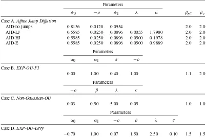
Table 1. Parameter setting for the Monte Carlo
Parameters
ψ0 −ρ ψ1 λ μ βσ2 βν
Case A.Affine Jump Diffusion
AJD-no jumps 0.8136 0.0128 0.0954 2.0 2.0
AJD-LJ 0.5585 0.0250 0.0896 0.0055 1.7980 2.0 2.0 AJD-HJ 0.5585 0.0250 0.0896 0.0500 0.1978 2.0 2.0 AJD-E 0.5585 0.0250 0.0896 0.0500 0.9889 2.0 2.0
Parameters
α0 α1 δ −ρ
Case B.EXP-OU-FI
0.00 1.00 0.40 1.00 1.1 2.0
Parameters
−ρ β λ c
Case C.Non-Gaussian-OU
0.03 0.50 5.00 0.05 1.0 1.0
Parameters
α0 α1 −ρ β λ c
Case D.EXP-OU-Lévy
−0.70 1.00 0.07 1.50 2.50 0.10 1.5 1.5
NOTE: Affine Jump Diffusionmodel is given in (3.1) with Lévy density of the jump process equal toλe−μx/μ1{x>0}(compound Poisson
process with exponentially distributed jumps).EXP-OU-FImodel is given in (3.3) with driving process being the fractional Brownian motion
Bδ,t.Non-Gaussian-OUmodel is given in (3.2) with Lévy subordinator having Lévy density given byce−λx
xβ+11{x>0}(tempered stable process).
EXP-OU-Lévymodel is given in (3.3) with Lévy density of the pure-jump driving Lévy process equal toce−λ|x|
|x|β+1(tempered stable process).
the 5-minute price increments bigger in absolute value than the truncation level (c=1.50), and then aggregate to 10-minutes and compute the power variation from them (without any fur-ther truncation). Finally, using the power variations over the two frequencies, we compute the activity signature function
for interval t using (4.4). Since it is impossible to report in any sensible manner each of the activity functions bX,t(p), a summary measure based on robust methods needs to bo com-puted: the quantile activity signature function defined in (4.5) and the quartilesq=0.25,0.50,0.75, commonly used in statis-tics, prove informative.
Recall in presence of jumps
bX,t(p)
P
−→max(β,p),
from the asymptotic analysis. So, in finite samples we expect the median QASF,B0.50(p), to be close toβfor powersp< β,
close topforp> β, and curvilinear forpin a neighborhood of β. The upper and lower QASFsB0.75(p)andB0.25(p)provide
an indication of sampling dispersion.
As a check, we compute the QASFs on simulated realiza-tions for a few well-known volatility models where the value of β is given. These simulated realizations follow standard con-ventions with annualized volatility based on 252 trading days per year. We simulate the different volatility models over a total of 4400 days, which corresponds to 200 months. Of course the activity level, which recall we just denoteβ here, is the same for all simulated months, but that need not be the case with ob-served data.
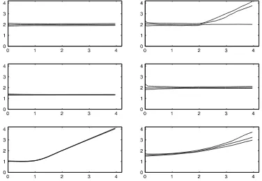
We start with an affine jump diffusion where the QASFs are shown in the top left and right-hand rows of Figure 1. In the top left, jumps are suppressed (Case AJD-no-jumps), the process is continuous, and the QASFs are flat aroundβ=2 as expected. In the top right (Case AJD-E) large rare jumps are added in to the Brownian diffusion. Now the QASFs are flat aroundβ=2 forp≤2, since the continuous component dom-inates here, while for p>2 the curves slope upwards to the asymptotic value p. The sharp break in slope atp=2 in the top right plot in Figure1is due to the dominance of the large jumps; this behavior might be unlikely in practice where only few months can have such big jumps, and the plots therefore should be regarded as a robustness check.
The plots in the second two rows in Figure 1 pertain to a Brownian long memory stochastic volatility with parameter set-tings B in Table1. To contrast the different activity of the spot variance and the VIX index in this model, we calculate also the QASFs of the unobservable spot variance. In the second row left-side are the QASFs for the simulated spot variance process, which are flat, reflecting continuity of the process, but around a value well less than 2.0. The reason is that the spot variance is not a semimartingale so there is no constraint that its QASF as-ymptotically pass through the point(2,2). The height of the as-ymptotic value of the activity signature function is determined by the fractional difference parameterd. Interestingly, for the second row right-hand side the QASFs for the VIX index asso-ciated with this spot volatility process are flat lines around 2.0, which has to be the case asymptotically because the VIX is a
Figure 1. QASFs for various stochastic volatility models. In each panel the three quantiles that are displayed are the 25th, 50th, and 75th, and are computed on the basis of 200 months of simulated data. The top left and right panels correspond to the AJD-no jumps and AJD-E, respec-tively, models. The middle panels correspond to the EXP-OU-FI model. The bottom left and right panels correspond to the Non-Gaussian-OU and EXP-OU-Lévy, respectively, specifications. All model specifications are given in Table1. In all cases but the middle right panel, theQASFs are based on the VIX index.QASFs for the middle-left panel are for the spot variance series. The truncation level in all cases isc=1.5.
portfolio of traded securities and thereby must be a semimartin-gale.
Finally, the two plots in the bottom row pertain to mod-els where volatility is a pure-jump process with no continuous component. The plot in the lower left of third row, pertains to the non-Gaussian OU modelCase Cin Table1. The value ofβ of the driving Lévy process is 0.50, but the bend occurs around
p=1.0. The reason is that the non-Gaussian OU model has a drift component, which must have an activity index of 1.0, and the approach taken here always reveals the index of the domi-nant component. The plot in the lower right row pertains to the Lévy-driven OU process, Case Din Table 1whereβ=1.50. There is a soft bend around the true value ofp=1.50 and the jumps are quite apparent forp≥2.00. The softness bend around
p=1.50 indicates that for higher values of the index the plots are just indicative and will not reveal the actual value with high precision.
5.2 Assessment of the Activity Estimator
The Monte Carlo assessment of the accuracy of the estimator (4.6) for each of the cases is shown in Table2. We computed the estimator for 5-minute returns for a 6.5 hour day, pooled over a period of a “month” (comprised of 22 trading days) and replicated 1000 times. The power parameter isp=0.95, but the results are quite insensitive to the choice ofpof the range 0.50 to 1.00. Table2shows the median and the median absolute de-viation about the median as measures of central tendency and variability, respectively. The reported results include no trunca-tion (NT) and truncatrunca-tion (T) at levelcin (4.1).
Results for the affine jump diffusion are in the first four rows of Table2. The estimator without truncation (NT) is unbiased and reasonably accurate, except in the casesAJD-Eand AJD-E-JS, where rather large jumps have been added to the diffusion. The caseAJD-E-JSalways contains at least one large jump in each simulated month. We are very grateful to a referee for pointing out that such large jumps could impart a finite sam-ple downward bias. The truncation pointc=1.50 (recall VIX index is quoted in annualized percentage units) is very mild, as it eliminates only one or two large moves per period, but as seen from the table in the (T) column it properly corrects for the downward bias.
Overall, Table2suggests the estimator is quite well behaved, regardless of whether the jumps are finitely or infinitely ac-tive and of bounded or unbounded variation. The truncation has no essential effect in any of the infinite activity cases, and it is really needed only in finite samples to guard against huge large rare jumps (which asymptotically do not matter). The dis-persion measure suggests the estimator is accurate to within a range between±0.05 to±0.10.
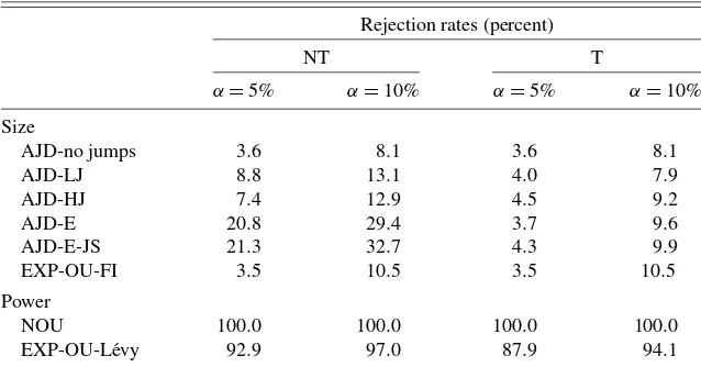
5.3 Assessment of the Test for a Brownian Component
We also evaluated the test for a Brownian component over the same set of replications and summarize the findings in Ta-ble3. For the first five cases of an affine jump diffusion, the null hypothesis is true, so the rejection rates represent the size of the test. Now it is seen that the truncation (T) is much more impor-tant for the actual size to agree closely with the nominal size. In the long memory model, the null is also true but the trunca-tion is irrelevant for this case. In the last two cases of pure jump volatility models the test is seen to have very high power.
Table 2. Small sample behavior ofβˆ
med(β)ˆ MAD
Case β NT T NT T
AJD-no jumps 2.00 2.01 2.01 0.081 0.079
AJD-LJ 2.00 2.00 2.01 0.086 0.079
AJD-HJ 2.00 1.98 2.00 0.081 0.081
AJD-E 2.00 1.92 2.00 0.093 0.082
AJD-E-JS 2.00 1.91 2.00 0.080 0.076
EXP-OU-FI 2.00 1.99 1.99 0.088 0.088
NOU 1.00 1.06 1.06 0.010 0.010
EXP-OU-Lévy 1.50 1.69 1.71 0.052 0.052
NOTE: Med is the median function; MAD=med| ˆβ−med(β)ˆ|; NT indicates no truncation; T indicates trun-cation withc=1.5; case AJD-E-JS is the same as AJD-E but we keep only simulations in which the estimation period contains at least one jump. There are 1000 replications of one month’s worth of 5-minute observations. The estimatorβis given in (4.6) forp=0.95.
6. EMPIRICAL APPLICATION
We use high-frequency data on the VIX index computed by the CBOE along with S&P 500 index futures returns. The dataset spans the period from September 22, 2003 until De-cember 31, 2008, for a total of 1212 trading days which cor-responds to 64 calendar months. Within each day, we use 5-minute records of the VIX index and the S&P 500 futures con-tract from 9.35 till 16.00 (EST) corresponding to 78 price ob-servations per day.
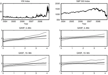
Table4shows simple summary statistics and the top two pan-els of Figure2 show plots of the high-frequency series. The sample moments of the series as shown in Table4are not sur-prising in view of the fact that the VIX is nonnegative, posi-tively autocorrelated, and right-skewed, together with the fact that the sample includes the very volatile year 2008. The sta-tistics on the ratio of the daily realized variance (RV) at the 5-minute and 10-minute levels are a check on possible mi-crostructure noise, since RV should be invariant to the sampling frequency in the absence of noise. These statistics suggest that noise is unlikely to be much of a problem but we need to be just a little guarded in interpreting the results for the S&P futures returns.
The paths of both VIX and S&P 500 index series exhibit dis-continuities. We tested the null hypothesis that in each month there is at least one jump using the test ofAit-Sahalia and Jacod (2009b), where we stress our alternative is of no jumps. At the 5% level of significance we can reject the null of the presence of jumps in only 14 and 23 months, respectively, for the VIX and the S&P 500 index.
6.1 How Active Are Stock Market Volatility and Returns?
To address these questions we start by displaying the Quan-tile Activity Signature Function (QASF) for each series, com-puted as developed in Todorov and Tauchen (2010a) for the 25th, 50th, and 75th quantiles. The unit interval used in the computation of the ASFs, as well as the rest of the statistics based on them, is a calendar month. The QASFs for 5-minute sampling are shown in the middle panels of Figure2with the VIX on the left and the S&P futures index on the right.
The contrasts between the VIX and the S&P index QASFs are small but quite noteworthy. The median and 75th QASFs for the VIX series on the left are just below 2.00 for powerspup to
Table 3. Size and power of the test for a Brownian component
Rejection rates (percent)
NT T
α=5% α=10% α=5% α=10%
Size
AJD-no jumps 3.6 8.1 3.6 8.1
AJD-LJ 8.8 13.1 4.0 7.9
AJD-HJ 7.4 12.9 4.5 9.2
AJD-E 20.8 29.4 3.7 9.6
AJD-E-JS 21.3 32.7 4.3 9.9
EXP-OU-FI 3.5 10.5 3.5 10.5
Power
NOU 100.0 100.0 100.0 100.0
EXP-OU-Lévy 92.9 97.0 87.9 94.1
NOTE: Case AJD-E-JS is the same as AJD-E but we keep only simulations in which each estimation period contains at least one jump. The rejection rates are based on 1000 replications of one month’s worth of 5-minute observations. In the construction of the testp=0.95. NT indicates no truncation; T indicates truncation with
c=1.5.
Table 4. Summary statistics for the data
Statistics VIX index S&P 500 index
Mean 18.26 −2.94
Std 10.52 20.84
Skewness 3.28 −0.89
Kurtosis 15.02 28.47
5-min autocorrelation 0.07 −0.03
quant0.25(RV10/RV5) 0.87 0.82 quant0.50(RV10/RV5) 1.00 0.94 quant0.75(RV10/RV5) 1.13 1.04
NOTE: The mean and standard deviation of the S&P index daily returns are annualized by multiplying by 252, respectively√252, and are reported in percentage terms. The statistics on realized variation (RV) are the quartiles of the ratios of daily RV at the 10 and 5-minute frequencies.
about 1.90, which would be expected for a pure jump process with a relatively high activity level around in the range 1.60– 1.90 or so. On the other hand, for the S&P index the QASF is centered right on 2.00 for powers up to 2.00, which would be expected of a process comprised of a Bronian diffusion plus jumps. These indications appear to be consistent over sampling interval, since the plots in the lower two panels of Figure2for the 10-minute frequency appear similar to the two middle pan-els.
Visual impressions notwithstand, we need to examine both the point estimates of the activity levels and the formal test for the presence or absence of a continuous component. We do this across the range of powers p=0.50,0.70,0.95. On Figure 3 we also plot a scatter of the activity estimates, cor-responding top=0.95, for the two series and all months in the
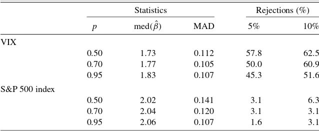
sample. The left-hand sides of Table5show the medians of the monthly point estimates along with the median absolute devia-tion about the median (MAD). The estimates indicate that the activity index for the VIX is in the range 1.73–1.83 and essen-tially exactly 2.00 for the S&P index; interestingly, the preci-sion level of±0.10 is consistent with that found in the Monte Carlo work for this sampling frequency. The right-hand side of Table5shows the outcomes, that is, the the rejection rates, for the formal test for the absence of a continuous component, which is derived inTodorov and Tauchen(2010a) and based on our estimator of the activity index. The rejection rates are for three values ofpbetween 0.50 and 1.00. The null hypothesis of the test is that the underlying process contains continuous mar-tingale plus possibly jumps, where perforce the index is 2.00. The alternative is that the underlying process lacks a
continu-Figure 2. Activity estimation results. The left panels correspond to the VIX index and the right ones to the S&P 500 index. The top two panels plot the high-frequency data. The middle panels reportQASFs for 5-minute sampling frequency and the bottom panels for 10-minute sampling frequency. TheQASFs are computed using 64 monthlyASFestimates for the sample period September 2003 till December 2008. The quantiles that are displayed are the 25th, 50th, and 75th. The truncation level for both series isc=1.5 The dashed lines in the two left bottom panels are straight lines at 2.
Figure 3. Scatterplot of the activity estimates. The estimates of the activity index correspond top=0.95 and truncationc=1.5.
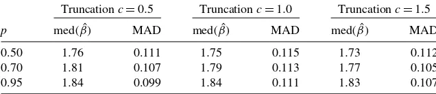
ous martingale and the index is thereby less than 2.00, so the test is one sided. Small values of the log of the estimator rel-ative to log(2.00)discredit the null hypothesis. In Table5, for the VIX the test rejection indicates no continuous component in half of the periods atp=0.70 with similar rejection rates for the other values ofp, while for the S&P 500 index the rejection rates always lie below the nominal significance level of the test. Since the truncation level cused in computingbX,t(p)is a tuning parameter, it is essential to assess the sensitivity of our key finding regarding the activity level of the VIX index with re-spect to the choice of the truncation point. Until now in the em-pirical analysis, as in the Monte Carlo study, we have used very mild truncation corresponding to removing on average only one high-frequency increment per month. In Table6we report also estimation results for other choices ofcthat result in a much more severe truncation. As seen from the table, our findings re-garding the volatility activity seem reasonably insensitive to the choice ofc.
To summarize, the evidence suggests that the VIX index is a pure-jump process without a continuous component and a rela-tively high activity index. The S&P 500 index itself, in contrast, is clearly a continuous plus jump process, which is consistent
with findings in other studies regarding the characteristics of fi-nancial price indices (Todorov and Tauchen 2010aand the ref-erences therein).
To the extent our evidence can be confirmed by future re-search, there would be important implications for modeling of the spot stochastic volatility process {σt2}. First, the ab-sence of a continuous component suggests that models such as the CGMY model are potentially plausible volatility mod-els, and the pricing of volatility derivatives would be substan-tially model complicated as noted inCont and Tankov(2004), section III, pp. 245–494. Second, affine jump diffusions appear unlikely candidates for volatility, since the contrast between the top right panel of Figure1and the middle-left and bottom-left panels of Figure2, together with the results in Table5, suggest that this sort of model was unlikely to have generated the data. The same contrast appears for the other affine jump diffusion specifications of Table1, whose QASF plots are not shown for reasons of space. Third, the pure-jump models of Barndorff-Nielsen and Shephard (2001) would also be unlikely candi-dates. The driving Lévy process for these models must have an activity index less than unity, and the volatility series itself will have an activity index of at most unity due to the drift, which dominates, and we estimate activity levels well above
Table 5. Estimates ofβXand tests for a Brownian component
Statistics Rejections (%)
p med(β)ˆ MAD 5% 10% VIX
0.50 1.73 0.112 57.8 62.5
0.70 1.77 0.105 50.0 60.9
0.95 1.83 0.107 45.3 51.6
S&P 500 index
0.50 2.02 0.141 3.1 6.3
0.70 2.04 0.120 3.1 3.1
0.95 2.06 0.107 1.6 3.1
NOTE: The median, MAD=med| ˆβ−med(β)ˆ|, and the rejection rates for the test are computed using 64 monthly estimates and tests for the sample period September 2003 till December 2008. The truncation used for both series isc=1.5.
Table 6. Robustness of estimatedβXfor VIX index with respect to truncation levelc
NOTE: Notation as in Table5. Truncationc=0.5 corresponds to 3.57 standard deviations for a 5-minute intraday change in the VIX index in our sample.
unity. The most plausible class of models would seem to be the
EXP-OU-Lévy discussed in Section3, since these models can ensure positivity and accommodate a pure jump model with ac-tivity indices above unity, as we find in the data.
Finally, we should point out that our conclusions about the volatility modeling rely on an estimate for the VIX index activ-ity, which although less than 2, is nevertheless still very close to it. Therefore, our estimation results can potentially still be gen-erated from a volatility process with a continuous martingale in it. However for this to happen, given our robustness checks of the estimation procedure, the continuous martingale should have a relatively small contribution in the power variation at the 5-minute frequency (asymptotically, i.e., as we sample more frequently, the continuous martingale will eventually dominate the power variation). This is not the case for most parametric jump-diffusion volatility models used to date as we illustrated in our Monte Carlo. Thus, at the very least, our results indi-cate that jumps play a much more prominent role in volatility modeling.
6.2 Are Market Volatility and Price Jumps Related?
Having detected the presence of jumps both in the S&P 500 index and the VIX index, a natural question arises about their dependence. We address this question in this section using the nonparametric tests developed in Jacod and Todorov(2009). Before presenting the tests and applying them to our dataset, we briefly summarize previous findings based on parametric or semiparametric specifications. As mentioned in the introduc-tion, the most commonly used model in finance which allows for jumps both in the price and the stochastic volatility is the double-jump model of Duffie, Pan, and Singleton (2000). In their general specification, Duffie, Pan, and Singleton (2000) allow for independent as well as dependent jumps in the index and its stochastic volatility. The studies that estimate double-jump models restrict them to arrive always together; see, for example,Chernov et al.(2003),Eraker, Johannes, and Polson (2003). These papers, however find that the correlation between the jump sizes in the price and volatility is not statistically different from zero. On the other hand, using high-frequency data and in the context of a pure jump model for the volatility, Todorov (2010) finds strong semiparametric evidence for de-pendent price and volatility jumps although perfect dependence is rejected.
Determining whether the jumps in the price and volatility ar-rive together and if so whether they are dependent is crucial from the perspective of successful risk management and con-sistent derivative pricing; see, for example,Cont and Kokholm
(2009), as well as for determining the volatility and jump risk premia. Therefore, here we investigate this important question in a completely nonparametric framework. In doing so we rely on the VIX data and Theorem1(b) linking the jump times of the VIX and the spot variance.
First, we investigate whether the jumps in the S&P 500 index and the VIX index arrive at the same time. For this, following Jacod and Todorov(2009), we use the following test statistic defined for two arbitrary processesXandY observed over the time interval(t−1,t)at frequency n
Tcj(t)=Vt(X,Y,2,2 n)
Vt(X,Y,2, n)
, (6.1)
whereVt(X,Y,r, n)is the following analogue of the realized power variation in a two-dimensional context
Vt(X,Y,r, n)=
If there is common arrival of jumps in X and Y over the in-terval(t−1,t], then this statistic converges to 1 (as n→0), while if the jumps in the two series never arrive together the limiting value of Tcj(t) is “around” 2. The intuition for that is that when common jumps are present then Vt(X,Y,2, n) and Vt(X,Y,2, n) converge to the same limit (which is
s∈[t−1,t)| Xs|2| Ys|2). Under the alternative of no common jumps, as for the univariate results in (4.3), we will need rescal-ing ofVt(X,Y,2, n)(which will depend on n) in order for it not to degenerate to zero (or infinity). For more details we refer toJacod and Todorov(2009).
We calculatedTcj for each day in our sample. The median value ofTcjis 1.389, which is relatively close to the value of 1, corresponding to common arrival of jumps in the price and the stochastic volatility. More formally, we also conducted a formal test usingTcj and the testing procedure outlined in Jacod and Todorov(2009). For 5 percent significance we failed to reject the null of common arrival of jumps in 838 out of the 1212 days in the sample.
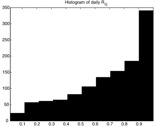
Another useful statistic that allows us to analyze cojump-ing in market volatility and market price level is the “realized” correlation between the squared jumps in those two series. For two arbitrary processesXandYobserved over the time interval (t−1,t)at frequency n, the realized correlation is defined as
Rcj(t)=
Vt(X,Y,2, n)
√
Vt(X,4, n)Vt(Y,4, n)
. (6.3)