Full Terms & Conditions of access and use can be found at
http://www.tandfonline.com/action/journalInformation?journalCode=ubes20
Download by: [Universitas Maritim Raja Ali Haji] Date: 13 January 2016, At: 00:39
Journal of Business & Economic Statistics
ISSN: 0735-0015 (Print) 1537-2707 (Online) Journal homepage: http://www.tandfonline.com/loi/ubes20
Business Cycle Asymmetries
Michael P Clements & Hans-Martin Krolzig
To cite this article: Michael P Clements & Hans-Martin Krolzig (2003) Business Cycle Asymmetries, Journal of Business & Economic Statistics, 21:1, 196-211, DOI: 10.1198/073500102288618892
To link to this article: http://dx.doi.org/10.1198/073500102288618892
View supplementary material
Published online: 01 Jan 2012.
Submit your article to this journal
Article views: 107
View related articles
Business Cycle Asymmetries:
Characterization and Testing Based
on Markov-Switching Autoregressions
Michael P.
Clements
Department of Economics, University of Warwick, Coventry CV4 7AL,
U.K. (M. P. clements@warwick.ac.uk)
Hans-Martin
Krolzig
Economics Department and Nuf’eld College, University of Oxford,
Oxford OX1 3UQ, U.K. (hans-martin.krolzig@nuf.ox.ac.uk)
Tests for business cycle asymmetries are developed for Markov-switching autoregressive models. The tests of deepness, steepness, and sharpness are Wald statistics, which have standard asymptotics. For the standard two-regime model of expansions and contractions, deepness is shown to imply sharpness (and vice versa), whereas the process is always nonsteep. Two and three-state models of U.S. GNP growth are used to illustrate the approach, along with models of U.S. investment and consumption growth. The robustness of the tests to model misspecication, and the effects of regime-dependent heteroscedasticity, are investigated.
KEY WORDS: Deepness; Regime-switching; Steepness and sharpness; Wald tests.
1. INTRODUCTION
: : :the most violent declines exceed the most considerable advances: : :. Business contractions appear to be a briefer and more violent process than business expansions.
—W. C. Mitchell (1927, p. 290)
There has been much interest in whether macroeconomic variables behave differently over the phases of the business cycle. Sichel (1993, p. 224) dened an asymmetric cycle as “one in which some phase of the cycle is different from the mirror image of the opposite phase.” McQueen and Thorley (1993, pp. 342–343) and Sichel (1993, pp. 225–226) discussed the importance, from both theoretical and empirical view-points, of establishing whether there are asymmetries in the business cycle. The nding of asymmetry is compatible with a number of business cycle models, but would rule out lin-ear models with symmetric errors. Sichel noted that models of asymmetric price adjustment can generate deepness (dened later), and referenced work of De Long and Summers (1998) and Ball and Mankiw (1994). More recently, the “output-gap” literature (see, e.g., Laxton, Meredith, and Rose 1995; Clark, Laxton, and Rose 1996) suggested that more of the adjustment in response to a negative demand shock falls on output than on prices, compared with the response to positive shocks. Finally, Sichel referenced models where entry to an industry is more costly than exit, which could result in steepness asymmetries. A number of types of asymmetry have been discussed in the literature. Primary types are steepness, deepness, and sharp-ness, or turning point (TP) asymmetry (henceforth termed SDS), which are typically tested for using separate nonpara-metric (NP) tests. Other types of asymmetries have been explored in parametric models, including asymmetric persis-tence to shocks (see Beaudry and Koop 1993; Hess and Iwata 1997a), and business cycle duration dependence (see, e.g., Sichel 1991; Diebold, Rudebusch, and Sichel 1993; Filardo 1994, Filardo and Gordon 1998). Our aim in this article is to analyze the conditions under which the Markov-switching
autoregressive (MS-AR) model class is capable of generating SDS asymmetries. The conditions are expressed as restric-tions on the parameters of the MS-AR model, which, if they held, would rule out a particular type of asymmetry. We then derive tests of these restrictions based on estimated MS-AR models, providing parametric tests as alternatives to the NP tests typically used in the literature. Our tests are able to detect asymmetries in the propagation mechanisms of shocks, or rst-moment asymmetries, whereas NP tests are unable to discriminate between rst-moment asymmetries and asymme-tries in the shocks. Since the work of Hamilton (1989), the MS-AR model class has been used extensively in the empiri-cal macroeconomics literature to analyze business cycle phe-nomena, and availability of good estimation and inferential procedures makes it an obvious choice for the development of parametric tests of asymmetry.
The basic MS-AR model at the center of our analysis is as follows. A stationary time series8xt9is assumed to have been
generated by an AR(p) with M MS regimes in the mean of the process, which we label an MSM(M)-AR(p) process,
xtƒŒ4st5D p X
kD1
k4xtƒkƒŒ4stƒk55Cut1
ut—st¹NID401‘250 (1)
We can order the regimes by the magnitude of Œ such that Œ1<¢ ¢ ¢< ŒM. The Markov chain is ergodic, irreducible, and there does not exist an absorbing state, that is, Nm 240115
for all mD11 : : : 1 M, where Nm is the ergodic or
uncondi-tional probability of regime m. The transition probabilities
©2003 American Statistical Association Journal of Business & Economic Statistics January 2003, Vol. 21, No. 1 DOI 10.1198/073500102288618892
196
are time-invariant,
pijDPr4stC1Dj—stDi51
M X
jD1
pijD11 8i1 j2811 : : : 1 M 91 (2)
so that the probability of a switch between regimesi andj does not depend on how long the process has been in regime i. A number of authors (including Diebold et al. 1993, Filardo 1994, Filardo and Gordon 1998) have extended the Hamilton (1989) model to allow for time-varying transition probabilities. Generally there appears to be positive duration dependence in contractions in the U.S. post-World War II period, so that the probability of moving out of recession increases with the duration of recession. However, nonconstant transition proba-bilities would complicate derivation of the SDS tests.
The MS-AR framework can be readily extended to mul-tivariate settings (see, e.g., Ravn and Sola 1995; Diebold and Rudebusch 1996; Hamilton and Lin 1996; Krolzig 1997; Krolzig and Sensier 2000; Krolzig and Toro 1998), which is a distinct advantage given that business cycles were origi-nally viewed as consisting of comovements in many economic variables (see, e.g., Burns and Mitchell 1946). In (1), xt can be a vector of variables. The extension of our tests to mul-tivariate settings, and models that include regime-dependent heteroscedasticity and switches in intercepts, are discussed in Section 4.
Along with constructing tests of asymmetries, a related goal is to establish precisely which types of asymmetries that MS-AR models are capable of generating in principle, given the widespread popularity of these models in applied research and the apparent confusion on this point in the literature. For example, Sichel (1993, p. 232, footnote 19) stated that the Hamilton (1989) two-state model implies steepness in U.S. GNP. In fact, steepness (as dened formally later) cannot arise in such a model. Recently, Hess and Iwata (1997b) have inves-tigated by simulation whether empirically estimated models, including MS-AR models, are able to replicate the “funda-mental business cycle features” of observed durations and amplitudes of contractions and expansions. Our focus is differ-ent, because we ask whether in principle MS-AR models can generate certain asymmetric features, in addition to whether empirically estimated models have these features.
Finally, because measures of economic activity exhibit sec-ular increases, the asymmetries relate to the detrended log of output. For example, Speight and McMillan (1998) consid-ered the detrended component (xt) of the variableyt, where xtDytƒ’t. Here’t is a nonstationary trend component, and xt is stationary, possibly consisting of cycle and noise compo-nents. Throughout the article,xtrefers to the detrended series. We assume that the nonstationarity can be removed by dif-ferencing, that is,xtDãyt. Trend elimination by differencing is natural in our setup, because the MS-AR model is typi-cally estimated on the rst difference of the log of output. An exception is the approach of Lam (1990), which allows for a general AR process in the level of the log of output, rather than imposing a unit root. However, none of the propositions on asymmetries in MS-AR models that follow, nor the testing
procedures, requires this method of detrending, and all remain valid whichever method is used. All that we require is that a MS-AR model can be estimated for the detrended series, how-soever obtained. The sensitivity of the ndings of asymmetries to the method of trend elimination requires further research. Gordon (1997) showed that in general the model of the short-run uctuations in output may depend on the treatment of the trend component.
The article is organized as follows. Section 2 reviews the literature on testing for business cycle asymmetries and shows how (the absence of) SDS asymmetries can be mapped into parameter restrictions of MS-AR models, paying par-ticular attention to the empirically relevant two- and three-regime models. Then, Section 3 derives the Wald tests of SDS hypotheses. Wald tests obviate the need to estimate the restricted (null) MS-AR model and are attractive for that rea-son. Section 4 shows how the basic testing approach can be extended in a number of directions. Section 5 uses Monte Carlo simulations to investigate the small-sample properties of the tests, their performance in the presence of heteroscedastic-ity, and their robustness to model misspecication. Section 6 sets out the empirical illustrations, and Section 7 concludes.
2. BUSINESS CYCLE ASYMMETRIES
2.1 A Brief Review of the Literature on Business
Cycle Asymmetries
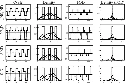
2.1.1 Steepness and Deepness. Sichel (1993) distin-guished two types of business cycle asymmetry: “steepness” and “deepness.” The former relates to whether contractions are steeper (or less steep) than expansions; the latter, to whether the amplitude of troughs exceeds (or is shallower than) that of peaks. The top left panel of Figure 1 depicts a schematic business cycle that is nondeep and nonsteep. The second panel in the rst column shows deepness of troughs (but nonsteep-ness), the third panel shows steepness of expansions (but nondeepness), and the last panel shows both properties.
A number of ways of testing for steepness and deepness have been proposed in the literature. Neftci (1984) proposed a test of whether there are longer runs of increases than decreases in a series, indicating that the length of expansions exceeds that of contractions, so that contractions are necessar-ily steeper than expansions. He dened an indicator variable ItD1 ifxt>0 (expansion) andItD ƒ1 ifxtµ0 (recession). Suppose thatIt can be represented by a second-order Markov process; then p22 > p11 (where p22 DPr6It D1—Itƒ1D11
Itƒ2D17andp11DPr6ItD ƒ1—Itƒ1D ƒ11 Itƒ2D ƒ17) implies a form of cylical asymmetry because the length of expansions exceeds that of contractions. A possible problem with this procedure is its sensitivity to noise. If increases (decreases) are inadvertently measured as decreases (increases), then the counts of transitions from which the estimates of the tran-sition probabilities are derived will be affected. Using this approach, Neftci found evidence of steepness in postwar U.S. unemployment during contractions. In contrast, Falk (1986) failed to nd evidence of steepness in other U.S. quarterly macroeconomic series using Neftci’s procedure, and Sichel (1989) suggested an error in Neftci’s work and indicated that
0 50 100 2
0
2
Cycle
N
S
,
N
D
2 1 0 1 2 0.5
1.0
Density
0 50 100 2.5
0.0 2.5
FOD
2.5 0.0 2.5 2.5
5.0
Density (FOD)
0 50 100 2
0 2
N
S
,D
2.5 0.0 2.5 0.25
0.50
0 50 100 2.5
0.0 2.5
2.5 0.0 2.5 1
2 3
0 50 100 2
0 2
S
,N
D
2 1 0 1 2 0.5
1.0
0 50 100 2.5
0.0 2.5
2.5 0.0 2.5 2
4 6
0 50 100 2
0 2
S
,D
2.5 0.0 2.5 0.25
0.50
0 50 100 2.5
0.0 2.5
2.5 0.0 2.5 1
2 3
Figure 1. Schematic of Business Cycle Asymmetries. The ’gure depicts four stylised business cycles. The ’rst row presents representations of a nonsteep, nondeep (NS, ND) cycle, the second row a nonsteep but deep cycle (NS, D), where contractions are deeper than expansions, the third row a steep (of expansions) but nondeep cycle (S, ND), and the fourth row a cycle that is steep and deep (S, D). For each row, the ’rst column depicts the time path for detrended output seriesxt, denoted “Cycle”, the second column shows the histograms (dotted line)
and densities (solid lines) forxt, the third column (“FOD”, ’rst-order difference) gives the time paths forãxt, and the fourth column gives the
histograms (dotted line) and densities (solid lines) forãxt. Two densities are drawn in the second and fourth columns, a density corresponding
to the histogram and a superimposed Gaussian curve.
the procedure might fail to nd steepness when in fact it is present. Rothman (1991) found evidence of asymmetry in the quarterly unemployment rate series using a modied version of Neftci’s test, and Sichel (1989) found strong evidence of asymmetry in annual unemployment, for which measurement error is presumably less important. Luukkonen and Ter¨asvirta (1991) noted that self-exciting threshold AR models (see, e.g., Tong and Lim 1980; Tong 1995) and smooth-transition AR models (see, e.g., Luukkonen, Saikkonen, and Ter¨asvirta 1988; Ter¨asvirta and Anderson 1992) may imply cyclical asymme-try in this sense, in that the probabilities of remaining in the regimes, once entered, may not be equal due to different dynamic structures.
Sichel (1993) suggested a test of deepness based on the coefcient of skewness calculated for the detrended series 8xt9. Deepness of contractions will show up as negative
skew-ness, because it implies that the average deviation of observa-tions below the mean will exceed that of observaobserva-tions above the mean. Steepness (of expansions) implies positive skewness in the rst difference of the detrended series,8ãxt9; increases should be larger, though less frequent, than decreases. Figure 1 illustrates this. The second column depicts the histograms (and densities) for 8xt9 corresponding to the schematic business
cycles in the rst column. The densities are symmetric for the rst and third rows because the business cycles are nondeep; those in the second and fourth rows exhibit negative skewness because of the deepness of contractions. The third and fourth
columns depict the times series of8ãxt9and their histograms
(and densities) for the schematic business cycles depicted in the rst column. The densities are symmetric for the rst and second rows because the business cycles are nonsteep; those in the third and fourth rows exhibit positive skewness because of the steepness of expansions.
On the basis of these tests, deepness is found to character-ize quarterly postwar U.S. unemployment and industrial pro-duction, with weaker evidence for GNP, whereas only unem-ployment (of the three) appears to exhibit steepness. We also report these NP tests based on the coefcients of skewness in our empirical work. In addition, the concepts of nondeepness and nonsteepness are used to construct parametric tests based on the MS-AR model in (1), which we turn to after discussing the third notion of asymmetry.
2.1.2 Sharpness. Sharpness, or TP asymmetry, as intro-duced by McQueen and Thorley (1993), result if, for exam-ple, troughs are “sharp” and peaks more “rounded.” McQueen and Thorley presented two tests. The rst test is based on the magnitude of growth rate changes around National Bureau of Economic Research–dated peaks and troughs. The mean abso-lute changes are calculated for peaks and troughs separately, and the test for asymmetry is based on rejecting the null of the population mean changes in the variable at peaks and troughs being equal. McQueen and Thorley found the null of equal TP sharpness can be rejected for both the unemployment rate and industrial production. Their second testing procedure is
based on a second-order, three-state Markov chain. They dis-tinguished between contraction, moderate, and high (recov-ery) states. The hypothesis of Hicks (1950) that troughs are sharper than peaks corresponds to the probability of jump-ing from the contraction to high-growth state exceedjump-ing the probability of jumping directly from high growth to contrac-tion. “Complete” TP symmetry requires that these switches be equally likely, that switches to moderate growth from contrac-tion and from high growth be equally likely, and that move-ments to high growth and contraction from moderate growth be also equally likely. McQueen and Thorley again found evi-dence of sharpness asymmetry for postwar unemployment and industrial production, but the susceptibility of the test to noise became evident when they considered prewar industrial pro-duction and postwar agricultural unemployment. In both cases, quarterly volatility in the series interrupted runs of ones and threes, reducing the number of sharp TPs and the power of the test. Their second approach can be implemented directly in a MS-AR model.
2.2 Formal De’nitions of Asymmetries
For clarity, we formally dene the concepts of steepness, deepness, and sharpness.
Denition 1: Deepness (Sichel 1993). The process8xt9is said to benondeep(nontall) iffxt is not skewed,
E64xtƒŒx537D00
Analogously, we can dene steepness as skewness of the differences.
Denition 2: Steepness (Sichel 1993). The process8xt9is
said to benonsteepiffãxt is not skewed,
E6ãx3 t7D00
The business cycle literature indicates the possibility of neg-ative skewness ofxt and ãxt—thus steep and deep
contrac-tions. The opposite case is oftall(E64xtƒŒ537 >0) andsteep
(ãxt positively skewed) expansions.
Denition 3: Sharpness (McQueen and Thorley 1993). The process8xt9is said to benonsharpiff the transition
prob-abilities to and from the two outer regimes are identical,
pm1DpmM andp1mDpMm1
for allm6D11 M 1 and p1MDpM10
In a two-regime model, for example, nonsharpness implies thatp12Dp21. In a three-regime model, it requiresp13Dp31
as well as p12Dp32 and p21Dp23. When M D4, the
fol-lowing restrictions on the matrix of transition probabilities are required to hold for nonsharpness,
PD
2.3 Asymmetries in MS-AR Processes
We now present the restrictions on the parameter space of the MSM-AR model that correspond to the concepts of asymmetry. Proofs of these propositions are conned to the Appendix. Whereas the restrictions implied by sharpness fol-low immediately, testing for deepness and steepness is less obvious.
According to Denition 1, deepness implies skewness. Using the properties of the MS-AR dened in (1) and (2), the following necessary and sufcient moment condition results.
Proposition 1. An MSM(M)-AR(p) process isnondeepiff
M
unconditional probability of regimemandŒxis the uncondi-tional mean ofxt.
The expression (4) is a complicated third-order poly-nomial in the regime-dependent parameters of the pro-cess,Œ11 : : : 1 ŒM, and the unconditional regime probabilities,
N
11 : : : 1NMƒ1, which are nonlinear functions of the transition
parameterspij. Equation (4) is derived from the condition that thekth moment ofŒt (withkD3) equals 0, whereŒt is the Markov chain component of the process (see the Appendix),
E£
ForMD2, the problem becomes more tractable analytically. Example 1. Consider the case of the two-regime MSM(2)-AR(p) process. Invoking Proposition 1, the skewness of the Markov chain is given by
E£ is apparent that nondeepness,E6Œ3
t7D0, requires thatN1D05.
Hence the matrix of transition probabilities must be symmet-ric, p12Dp21. This also implies that the regime-conditional
meansŒ1andŒ2are equidistant to the unconditional meanŒx.
Hence, in the case of two regimes, nondeepness can be tested by testing the hypothesisp12Dp21. This is equivalent
to the test of nonsharpness. For processes withM >2, we pro-pose testing for nondeepness based on theΟ
m conditional on
Œx and theNm.
Example 2. Consider now an MSM(3)-AR(p) process. Again, by invoking Proposition 1, the skewness of the Markov chainŒt is given by
Nondeepness,E6Œ3
t7D0, requires that
We now derive conditions for the presence of steepness based on the skewness of the differenced series.
Proposition 2. An MSM(M)-AR(p) process isnonsteepif the size of the jumps,ŒjƒŒi, satises the following condition:
MXƒ1
Symmetry of the matrix of transition parameters (which is stronger than the denition of sharpness) is sufcient but not necessary for nonsteepness. A proof of this proposition appears in the Appendix.
In contrast with deepness, the condition for steepness depends not only on the ergodic probabilities,Nj, but also
directly on the transition parameters.
Example 3. In an MSM(2)-AR(p) process, condition (5) gives
Example 4. For an MSM(3)-AR(p) process, we get
E£
Although this is a complicated expression, the concept of steepness can be made operational by using the sufcient con-dition, that is, the symmetry of the matrix of transition param-eters, which implies nonsteepness. As noted earlier, this is stronger than the property of nonsharpness.
We close this section with a corollary characterizing the two-regime MS-AR model, which shows the impossibility of the MS(2)-AR exhibiting steepness and the equivalence of the concepts of deepness and sharpness.
Corollary 1. A two-regime MS model is always nonsteep. Nonsharpness implies nondeepness and vice versa.
Nonsteepness is evident from Example 3. BecauseN1=N2D
p21=p12, we have thatN1p12ƒ N2p21D0 and henceE6ãŒ3t7D
0. Further, nonsharpness (symmetric transition probabilities, p12Dp21) implies nondeepness,E64xtƒŒx537D0, and vice
versa. In particular, both concepts imply that the regime-conditional means Œ1 and Œ2 are equidistant to the
uncondi-tional meanŒx.
3. PARAMETRIC TESTS BASED
ON THE MARKOV-SWITCHING AUTOREGRESSIVE MODEL
Testing the MS-AR model against a linear null (or three regimes versus two regimes) is complicated due to the pres-ence of unidentied nuisance parameters under the null of linearity (i.e., the transition probabilities) and because the scores associated with parameters of interest under the alter-native may be identically 0 under the null. These issues have been looked at by a number of authors (see, e.g., Hansen 1992, 1996), but are not of direct interest to us here, because the number of regimes remains unchanged under all three asymmetry hypotheses, so that standard asymptotics can be invoked. But we note that in practice they may complicate identication of the appropriate model on which to carry out the asymmetry tests.
Wald tests of the asymmetry hypotheses are computation-ally attractive, because the model does not have to be esti-mated under the null. In general terms, we consider Wald (W) tests of the hypothesis
H02 ”4‹5D0 versus H12 ”4‹56D01
where ”2 òn !òr is a continuously differentiable func-tion with rank r, rDrk4¡”4‹5¡‹0 5µdim‹. Because the pij are
restricted to the 60117 interval, the tests are formulated on the logits ij Dlog4 pij
1ƒpij5, which avoids problems if one or
more of thepij is close to the border. It is worth noting that
if 1
eter is taken as xed and is eliminated from the parameter vector‹.
Let ‹Q denote the unconstrained maximum likelihood esti-mator (MLE) of‹D4Œ11 : : : 1 ŒM3 11 : : : 1 p1‘23Ï5, andO‹
the restricted MLE under the null. Then the Wald test statistic W is based on the unconstrained estimator‹Q, which is asymp-totically normal,
p
T 4‹Qƒ‹5!d N401 è‹Q51
where, for the MLE,è‹Q D=ƒa1 is the inverse of the
asymp-totic information matrix. This can be calculated numerically. It follows that”4‹5Q is also normal for large samples,
p
Thus if H02 ”4‹5D0 is true and the variance–covariance
matrix is invertible, then
T ”4‹5Q 0
The Wald test for the null of nondeepness is based on
”D4‹5D”D4Ï1Ì3¢5 2D
29 the Wald test statistic for
nondeepness is given by
T ”D4‹50
Example 5. ForMD2, the null of nondeepness is based on
Because this test is difcult to implement for M >2, for models with more than two regimes we use a version of the deepness test with Nm andŒx taken as xed. This Wald test
for the null of nondeepness is based on
”D24‹5D”D24Ì3¢5 2D
Example 6. ForMD3, the null of nondeepness is tested by”D24‹5D0 and so has the form
A Wald test for the null of nonsteepness can be based on
”S4‹5D”S4Ì3¢5 2D
test concerns only the vector of mean parameters,
ïÌD
and
¡‹i D0 otherwise. The Wald test statistic has the form
”4‹5Q 0
In the case of a three-state Markov chain, for example,
QD
The null of nonsharpness can be expressed as
”TP4‹5D”TP4Ï3¢5 2DêÏ1
the matrix of logit transition probabilities. Then the vector Ï is given by vecd4ç5, dened as vec4ç5with the diagonal elements ij excluded. In the case of a three-state Markov
chain, for example, we have that
ÏD4121 131 211 231 311 3250
For linear restrictions, the relevant Wald statistic can be expressed as
WTPDT 4ê‹Qƒ506êeè‹Qê07ƒ
1
4ê‹Qƒ50
Thus under the null of symmetric transition probabilities, the Wald statistic has the form
WTPD Q0ê0£
4. EXTENSIONS TO THE TESTING FRAMEWORK
In this section we outline three extensions to the basic framework for testing for asymmetries in MS-AR models. We deal with models in which the intercept, rather than the mean switches between regimes and models that display regime-dependent heteroscedasticity and consider multivariate set-tings.
4.1 Switching Intercepts
The MSI(M)-AR(p) model is characterized by switching in theintercept, rather than themean(MSM-AR),
xtDŒ4st5C
As in the MSM-AR process, the MSI(M)-AR(p) process can be written as the sum of two independent processes,
xtƒŒxDŒtCzt1 (9)
the contribution of the Markov chain andE6Œt7D0. To derive
an expression forŒt, rst rewrite (8) as equivalent to (8), the following expression forŒt is obtained:
ŒtDƒ14L5
t0 (11)
Thus, in contrast to the MSM-AR model considered so far, in which a shift in regime causes a once-and-for-all jump in the level of the observed time series, the MSI-AR model implies a smooth transition in the level of the process after a shift in regime.
Tests for asymmetries in MSI(M)-AR(p) models can be based ont, which can be seen to be equivalent to theŒt in
MSM(M)-AR(p) models. Wald tests for deepness and steep-ness can be easily constructed by applying the procedures developed in Section 3 to parametric tests for the skewness of t andãt.
A potential problem arises when the roots of4L5are close to the unit circle and, in the extreme, for the rst-order polyno-mial,4L5D1ƒL,D1. ThentDãŒt, and testingtfor
deepness leads to conclusions for the deepness ofãxt (rather
than xt). In other words, applying the conditions derived for
deepness in the MSM-AR model totprovides a test of
steep-ness of the MSI-AR model. In our examples, the roots of4L5 are a long way from unity because we are modeling rst dif-ferences, and these exhibit little dependence relative to models in levels. Furthermore, the extreme case of a unit root implies that the data have not been differenced a sufcient number of times before modeling.
4.2 Regime-Dependent Heteroscedasticity
In the original Hamilton model, the variance of the distur-bance term does not depend on the regime. However, regime-dependent heteroscedasticity is often manifest when the model is applied to nancial data and also perhaps (albeit to a lesser extent) to macroeconomic data. For example, Koop, Pesaran, and Potter (1996) found evidence of regime-dependent error variances in a nonlinear model of output growth and unem-ployment rate changes. Therefore, the assumption thatut—st¹ NID401‘25 in (1) may need to be replaced by u
t—st ¹ NID401‘24s
t55, where in a two-regime model, for example,
‘24s
t5D‘12whenstD1 and‘24st5D‘22whenstD2. In such
a model, asymmetries in the observed variable can arise either from asymmetries in the model’s propagation mechanism or from asymmetries in the innovations. Failure to allow for het-eroscedasticity in the MS-AR model when it is present in the data may affect the properties of the SDS tests, as shown in Section 5. Luukkonen and Ter¨asvirta (1991) tested for cycli-cal asymmetry by testing whether a linear AR model can be rejected in favor of a smooth-transition AR, and are concerned that asymmetry may result simply because of regime het-eroscedasticity. Consequently, these authors also tested for AR conditional heteroscedasticity. The SDS tests can be calculated within a model that explicitly allows for heteroscedasticity.
Our tests are designed to detect asymmetries in the model’s propagation mechanism, whereas the NP tests are unable to discriminate between the two sources of asymmetry.
4.3 Multivariate Models
The tests that we have outlined apply equally to a vector process with a single state variable. Models of this sort arise when the variables share a common cyclical component, as in the MS-VAR model of postwar U.S. employment and out-put of Krolzig and Toro (1998) or the dynamic-factor model with regime switching of Diebold and Rudebusch (1996). Note that the test of sharpness is intrinsically a system-based test, because it evaluates the transition probabilies of the common latent regime variable. In contrast, the tests for deepness and steepness (forM >2) focus on variable-specic asymmetries. It is therefore possible to test each variable for asymmetry.
In some instances, it may be appropriate to allow more than one state variable, as in the bivariate model of stock returns and output growth of Hamilton and Lin (1996), where each variable responds to a specic state variable. The procedures developed in Section 3 can then be applied in the same way, using the regime means and ergodic and transition probabili-ties relevant for each pairing of variable and state variable.
5. PROPERTIES OF TESTING PROCEDURES
In this section we explore by Monte Carlo (a) the size and power properties of our parametric tests relative to NP tests, (b) the impact on our testing procedures of ignoring regime-dependent heteroscedasticity, and (c) their properties under model misspecication, by which we mean applying the MS-AR model-based tests when the process was generated by an alternative model.
5.1 Size and Power
Table 1 reports the empirical sizes and powers of the tests from a Monte Carlo (based on 1,000 replications) for two data-generating processes (DGPs) based on
xtDŒ4st5C…t1 where …t¹NID401‘ 2
5 and st2811290
(12)
For the rst process, labeled “Symmetric MSM” in Table 1, Œ1D ƒŒ2D ƒ105,‘2D1, and p
11 Dp22D085. Thus, from
the propositions stated in Section 2.3, it is apparent that the values ofŒ4st5andN1 satisfy the conditions forŒt, and thus
xt, to exhibit nondeepness. (Nonsteepness is a property of the
model, and nondeepness implies nonsharpness in this model.) The parameter values for the second process, labeled “Asym-metric MSM,” are the same except that p11D065, and the
conditions for nondeepness do not hold.
Because the DGP consists of two regimes, there are no entries for our steepness test (MS:Steepness) in Table 1; such processes can not exhibit steepness. The NP test rejection fre-quencies for steepness (NP:Steepness) are close to the nomi-nal sizes for all of the DGPs. The test for sharpness has size close to nominal even forT D100, and power of nearly 60% at a 5% size. The parametric deepness test (MS:Deepness) is correctly sized asymptotically and only a little too large for TD100. Moreover, it has good power for the asymmetric pro-cess forT D100.
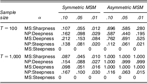
Table 1. Empirical Size and Power of Tests of Asymmetries
Symmetric MSM Asymmetric MSM
Sample
size .10 .05 .01 .10 .05 .01
TD100 MS:Sharpness 0107 0055 0012 0696 0585 0280 NP:Deepness 0162 0098 0029 0587 0440 0195 MS:Deepness 0212 0153 0084 0762 0691 0525 NP:Steepness 0138 0081 0020 0112 0061 0021
MS:Steepness 0 0 0 0 0 0
TD11000 MS:Sharpness 0087 0045 0010 10000 10000 10000 NP:Deepness 0154 0088 0027 10000 0999 0999 MS:Deepness 0098 0051 0016 10000 10000 10000 NP:Steepness 0167 0100 0030 0116 0063 0015
MS:Steepness 0 0 0 0 0 0
NOTE: This table records the rejection frequencies of tests for asymmetry at three nominal sizes (D01010051001) for a “symmetric” MS-AR DGP, and an “asymmetric” MS-AR DGP. The
former is nonsharp, nondeep, and nonsteep. The latter is deep. The rejection frequencies are empirical sizes for the symmetric DGP and powers for the asymmetric DGP.
MS:Deepness refers to the MS-AR parametric test of deepness; NP:Deepness, to the nonparametric test of deepness; and so on.
5.0 2.5 0.0 2.5 5.0 0.1
0.2 0.3 0.4
m1=-1.5, m2=1.5, s1=1, s2=1, Pr(s=1)=.5
5.0 2.5 0.0 2.5 5.0 0.1
0.2 0.3 0.4
m1=-1.5, m2=1.5, s1=1, s2=1, Pr(s=1)=.3
5.0 2.5 0.0 2.5 5.0 0.1
0.2 0.3 0.4
m1=-1.5, m2=1.5, s1=1, s2=2, Pr(s=1)=.5
5.0 2.5 0.0 2.5 5.0 0.1
0.2 0.3 0.4
m1=-1.5, m2=1.5, s1=1, s2=2, Pr(s=1)=.3
(a) (b)
(c) (d)
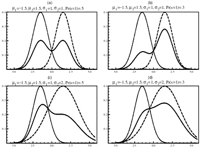
Figure 2. Asymmetries Due to Regime-Dependent Heteroscedasticity. The ’gure depicts densities (conditional on the regime and uncondi-tional) ofxt constructed for two-regime MS-AR models [- - - -p(x—sD1); – – –p(x—sD2); ——p(x)]. In (a), the MS-AR model satis’es the conditions for a symmetric propagation mechanism, and the process is homoscedastic. The unconditional density (the solid line) is symmetric. In (b), depicting a homoscedastic process with an asymmetric propagation mechanism, the unconditional density is skewed. The process in the (c) has a symmetric propagation mechanism but has regime-dependent heteroscedasticity. The unconditional density is skewed. The process in (d) has asymmetric innovations and an asymmetric propagation mechanism.
5.2 Robustness Under Heteroscedasticity
Our tests are designed to detect asymmetries in the Markov chain component,Œt, which we have termed “rst-moment asymmetry,” whereas the NP tests would be expected to reject the null of asymmetry in the presence of regime-dependent variances of the shocks (“heteroscedasticity”). The data-generating processes chosen to explore these issues is a simple extension of (12) to allow for heteroscedasticity,
xtDŒ4st5C…t1 where…t¹NID401‘24st55 and
st2811290 (13)
To illustrate, Figure 2 plots the density of xt generated by
(13) and the density conditional on being in a regime. In (a), Œ1D ƒŒ2D ƒ105, ‘2
1 D‘
2
2 D1, and Pr4stD15D05. From
the propositions stated in Section 2.3, it is apparent that the values ofŒ4st5andN1 satisfy the conditions forŒt, and thus
xt, to exhibit nondeepness. (Nonsteepness is a property of the
model.) The density exhibits skewness in (b) because the con-dition for nondeepness is not satised by Œ1D ƒŒ2D ƒ105
and Pr4st D15D03. In (c) the condition for nondeepness is
satised, becauseŒ1D ƒŒ2D ƒ105 and Pr4stD15D05, but nonetheless heteroscedasticity,‘2
1 D1 and ‘ 2
2 D2, induces
skewness inxt. So the contribution of the Markov process is
symmetric, but the unequal variances result in asymmetry in
the marginal distribution of xt. Figure 2(d) is akin to (b) but
with heteroscedastic errors.
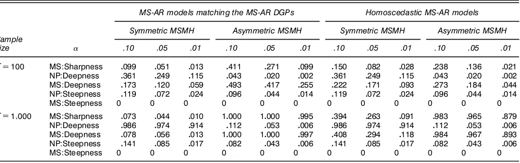
Table 2 reports the properties of the testing procedures for heteroscedastic MS-AR processes, when the estimated model allows for regime-dependent error variances. The NP test rejection frequencies for steepness (NP:Steepness) are close to the nominal sizes for all of the DGPs, so the presence of heteroscedasticity does not inate the size of the test. The test for sharpness has size close to nominal even forTD100. The power approximately halves when the DGP is heteroscedastic (compare the “Asymmetric MSMH” columns in Table 2 with the “Asymmetric MSMH” columns of Table 1), but as the entries for T D11000 conrm, this is a small-sample effect. The parametric deepness test (MS:Deepness) is correctly sized asymptotically and only a little too large forT D100. More-over, it has good power for the asymmetric DGP forT D100. In contrast, the NP (NP:Deepness) test is less powerful, has a size approaching 1 asymptotically for the symmetric MSMH, and has power approximately equal to size for a 5% test for the asymmetric MSMH whenT D11000.
The second aspect the Monte Carlo explores is the effect of using homoscedastic models when the DGP is heteroscedas-tic. Table 2 shows that the sizes of the parametric sharpness and deepness tests are a little inated for T D100 and are 25%–30% for a nominal size of 5% for the large sample.
Table 2. Empirical Size and Power of Tests of Asymmetries When There are Heteroscedastic Disturbances
MS-AR models matching the MS-AR DGPs Homoscedastic MS-AR models
Symmetric MSMH Asymmetric MSMH Symmetric MSMH Asymmetric MSMH
Sample
size .10 .05 .01 .10 .05 .01 .10 .05 .01 .10 .05 .01
TD100 MS:Sharpness 0099 0051 0013 0411 0271 0099 0150 0082 0028 0238 0136 0021 NP:Deepness 0361 0249 0115 0043 0020 0002 0361 0249 0115 0043 0020 0002 MS:Deepness 0173 0120 0059 0493 0417 0255 0222 0171 0093 0273 0184 0044 NP:Steepness 0119 0072 0024 0096 0044 0014 0119 0072 0024 0096 0044 0014
MS:Steepness 0 0 0 0 0 0 0 0 0 0 0 0
TD11000 MS:Sharpness 0073 0044 0010 10000 10000 0995 0394 0263 0091 0983 0965 0879 NP:Deepness 0986 0974 0914 0112 0053 0006 0986 0974 0914 0112 0053 0006 MS:Deepness 0078 0056 0013 10000 10000 0997 0408 0294 0118 0984 0967 0893 NP:Steepness 0141 0085 0017 0082 0043 0006 0141 0085 0017 0082 0043 0006
MS:Steepness 0 0 0 0 0 0 0 0 0 0 0 0
NOTE: The table records the rejection frequencies of tests for asymmetry at three nominal sizes,D01010051001, for two DGPs: a heteroscedastic MS-AR with a symmetric propagation mechanism, labeled “symmetric MSMH,” and a heteroscedastic MS-AR with an asymmetric propagation mechanism, labeled “asymmetric MSMH,” which is deep. For both DGPs,‘1D1,
‘2D2. For the symmetric MSMH,Œ1D ƒ105,Œ2D105, andp11Dp22D085; for the asymmetric MSMH,Œ1D ƒ105,Œ2D105,p11D065, andp22D085.
For each DGP, the table records the results of testing for asymmetries within MS-AR models that allow for the heteroscedasticity (the left half of the table) and in MS-AR models that impose equal error variances across the two regimes (the right half of the table). The rejection frequencies are empirical sizes for the symmetric MS-AR, and powers for the asymmetric MS-AR.
MS:Deepness refers to the MS-AR parametric test of deepness; NP:deepness, to the nonparametric test of Deepness; and so on.
Finally, the failure to model the heteroscedasticity reduces the power of the asymmetry tests for the DGP considered.
5.3 Robustness Under Model Misspeci’cation
Alternative regime-switching models have been proposed in the literature to explain business cycle phenomena. Because these models may in some instances provide a better char-acterization of the data than the MS-AR model, a relevant question is how well the parametric tests perform when the model on which they are based (i.e., the MS-AR model) is not the model that generated the data. In this section we report Monte Carlo simulations designed to investigate the properties of the proposed testing procedures under model misspecication. Results are recorded in Table 3 for a self-exciting threshold AR (SETAR) DGP and a smooth-transition AR (STAR) DGP. SETAR models have been estimated for U.S. output growth by a number of authors, including Tiao and Tsay (1994), Potter (1995), Pesaran and Potter (1997), and Clements and Smith (2000). A statistical analysis of the
Table 3. Empirical Size and Power: SETAR and LSTAR DGPs
MS-AR model applied to data from SETAR and LSTAR DGPs
Symmetric SETAR Asymmetric SETAR Symmetric LSTAR Asymmetric LSTAR
Sample
size .10 .05 .01 .10 .05 .01 .10 .05 .01 .10 .05 .01
TD100 MS:Sharpness 0116 0053 0010 0529 0429 0161 0114 0048 0010 0505 0404 0158 NP:Deepness 0398 0313 0169 0485 0428 0314 0390 0296 0158 0383 0313 0211 MS:Deepness 0306 0261 0193 0212 0137 0074 0324 0272 0192 0192 0113 0047 NP:Steepness 0057 0025 0007 0062 0027 0005 0067 0035 0008 0081 0038 0008
MS:Steepness 0 0 0 0 0 0 0 0 0 0 0 0
TD11000 MS:Sharpness 0077 0034 0004 0999 0998 0998 0062 0026 0003 0993 0992 0992 NP:Deepness 0410 0333 0186 0997 0993 0987 0384 0295 0183 0972 0958 0935 MS:Deepness 0113 0071 0020 0974 0926 0644 0096 0054 0017 0943 0854 0475 NP:Steepness 0073 0033 0010 0105 0046 0010 0089 0045 0016 0287 0160 0045
MS:Steepness 0 0 0 0 0 0 0 0 0 0 0 0
NOTE: The table records the rejection frequencies of tests for asymmetry at three nominal sizes (D01010051001) for four DGPs: symmetric and asymmetric SETAR models and symmetric
and asymmetric STAR models. ThecandƒDGP parameter vlaues are as follows: for the symmetric SETAR,cD0; for the asymmetric SETAR,cD ƒ075; for the symmetric STAR,cD0,ƒD10; and for the asymmetric STAR,cD ƒ075,ƒD10.
MS:Deepness refers to the MS-AR parametric test of deepness; NP:Deepness, to the nonparametric test of deepness; and so on.
SETAR model was provided by Tong (1995), and of the STAR model by Luukkonen et al. (1998) and Ter¨asvirta and Anderson (1992).
The regime-generating process in both models is not assumed to be exogenous, but rather directly linked to a tran-sition variable. For the SETAR model, the trantran-sition variable is a lag of the endogenous variable, say,xtƒd,
xtD
Á
Œ1C p X
iD1
1ixtƒi
!
41ƒI4xtƒd3 c55
C
Á
Œ2C p X
iD1
2ixtƒi
!
I4xtƒd3 c5C˜t1 (14)
where ˜t¹IID401‘25,I4xtƒd3 c5D1 ifxtƒd> c and 0
other-wise andc is the threshold at which the switching between regimes occurs.
In the STAR model, the weight attached to the regimes depends on the realization of an exogenous or lagged endogenous variablezt, so that the transition between regimes
is “smooth,”
xtD
Á
Œ1C p X
iD1
1ixtƒi
!
41ƒG4zt3 ƒ1 c55
C
Á
Œ2C p X
iD1
2ixtƒi
!
G4zt3 ƒ1 c5C˜t1 (15)
where ˜t¹IID401‘25 and the transition functionG4zt3 ƒ1 c5
is a continuous function, usually bounded between 0 and 1. We consider the LSTAR model, where the transition function is given by
G4zt3 ƒ1 c5D
1
1Cexp8ƒƒ4ztƒc591
where ƒ is the smoothness parameter and the transition vari-able zt is taken to be the lagged endogenous variable (zt D
xtƒd). For ƒ >0, as zt ! ƒˆ, G4¢5!0, and for zt! ˆ,
G4¢5!1.
To simplify matters, in our simulations we set1iD2iD0
for all i, dD1, ‘2D1, Œ
1D ƒŒ2D ƒ105, and vary c to
give symmetric and asymmetric models. The results in Table 3 demonstrate the excellent performance of the MS model-based sharpness test. Even for the small sample size of T D100, it has approximately the correct size under model misspeci-cation. It also has good power in small samples for both the asymmetric SETAR and LSTAR DGPs. In contrast, the para-metric and NP nondeepness tests work less well in small sam-ples, but for large samples the parametric nondeepness test (MS:Deepness) is only slightly oversized and is clearly better behaved than the NP one.
Overall, the Monte Carlo results support the use of the proposed tests for business cycle asymmetries. The tests (a) behave as expected for correctly specied MS models, (b) are robust against skewness due to heteroscedasticity, and have been found to be reliable tests for business cycle asymmetries even if the underlying DGP is different from the empirical model. The tests proposed in this article enhance the role of the MS model as a exible tool for empirical modelling.
6. EMPIRICAL ILLUSTRATIONS
The SDS tests are illustrated on a number of datasets. Specically, we apply the parametric tests discussed in Section 3 to the MS(2)-AR(4) model of output growth of Hamilton (1989) for his original sample period of 1953–1984, to the MS(3)-AR(4) model of Clements and Krolzig (1998) on more recent data, and to various models of U.S. investment and consumption growth. In each case, the outcomes of the tests for asymmetries are compared with NP tests of skewness.
6.1 The Hamilton Model of U.S. Output Growth
MS-AR models have been used in contemporary empirical macroeconomics to capture certain features of the business cycle, but the formal testing of asymmetries has been largely conned to NP approaches. The seminal article by Hamilton
(1989) t a fourth-order autoregression (pD4) to the quarterly percentage change in U.S. real GNP,xt, from 1953 to 1984,
xtƒŒ4st5D14xtƒ1ƒŒ4stƒ155C¢¢¢C44xtƒpƒŒ4stƒ455C…t1
(16)
where …t ¹ NID401‘25 and the conditional mean Œ4s t5
switches between two states, “expansion” and “contraction,”
Œ4st5D (
Œ1<0 if stD1 (“contraction” or “recession”)
Œ2>0 if stD2 (“expansion” or “boom”)1
with the variance of the disturbance term, ‘24s
t5D‘2,
assumed to be the same in both regimes. This is an MS mean model, with the autoregressive parameters and disturbances independent of the statest.
Maximization of the likelihood function of an MS-AR model entails an iterative estimation technique to obtain esti-mates of the parameters of the AR and the transition proba-bilities governing the Markov chain of the unobserved states. Hamilton (1990) presented an expectation maximization (EM) algorithm for this class of model, and Krolzig (1997) gave an overview of alternative numerical techniques for maximum likelihood estimation of these models.
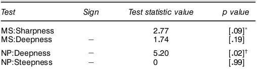
The results of testing for asymmetry based on the original Hamilton model and dataset (1952:2–1984:4) are recorded in Table 4. The NP test for skewness indicates signicant nega-tive skewness in output growth (i.e., deepness of contractions) at the 5% level. Our parametric test of nondeepness also indi-cates negative skewness, but is signicant only at the 20% level. There is evidence of sharpness at the 10% level, with the probability of switching from contraction to expansion exceed-ing the probability of movement in the reverse direction.
6.2 The Three-Regime Heteroscedastic Model
of U.S. Output Growth
Sichel (1994) argued that postwar business cycles typically consist of three phases: contraction, followed by high-growth recovery and then a period of moderate growth. To capture this in a parametric model, we consider the three-state MS-AR model of Clements and Krolzig (1998). This model consists of a shifting intercept term and a heteroscedastic error term and is denoted an MSIH(3)-AR(4) model, where H ags the
Table 4. Tests for Asymmetries Using the MSM(2)-AR(4) Model of U.S. Output Growth, 1952:2–1984:4
Test Sign Test statistic value pvalue
MS:Sharpness 2077 [009]ü
MS:Deepness ƒ 1074 [019]
NP:Deepness ƒ 5020 [002]†
NP:Steepness ƒ 0 [099]
NOTE: The NP and MS test statistics are2(1)under the null of symmetry. A positive (neg-ative) value of “Sign” ‘ags positive (neg(neg-ative) skewness. Nonsteepness is a property of the two-regime model; see Corollary 1.
üSigni’cance at the 10% level. †Signi’cance at the 5% level.
1950 1960 1970 1980 1990 0.5
1.0High-Growth Regime, H 1948:21990:4
1950 1960 1970 1980 1990 0.5
1.0 1948:21984:4
1950 1960 1970 1980 1990 0.5
1.0Recession Regime, L 1948:21990:4
1950 1960 1970 1980 1990 0.5
1.0 1960:21996:2
1950 1960 1970 1980 1990 0.5
1.0 1960:21990:4
1950 1960 1970 1980 1990 0.5
1.0 1948:21984:4
1950 1960 1970 1980 1990 0.5
1.0 1960:21996:2
1950 1960 1970 1980 1990 0.5
1.0 1960:21990:4
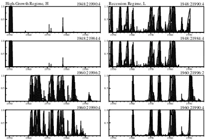
Figure 3. MSIH(3)-AR(4) Model of U.S. Output Growth: Smoothed (Solid Lines) and Filtered (Dashed Blocks) Probabilities of the High-Growth
H(left column) and “Recession”LRegime (Right column). Each row refers to a different historical period.
heteroscedastic error term and 3 and 4 refer to the number of regimes and AR lags. It is written as
xtDŒ4st5C 4
X
kD1
kxtƒkC…t1 (17)
where …t ¹NID4‘24s
t55 and st 28112139 is generated by a
Markov chain. The three-state model is preferred over the two-state model, because the latter does not always yield a good representation of the business cycle when tted to peri-ods outside that of Hamilton (1989) (see, e.g., Boldin 1996; Clements and Krolzig 1998). Clements and Krolzig (1998) found an average duration of contraction of 2–3 quarters when the two-state model is t to the period 1947–1990, and of less than 2 quarters when it is t for 1959–1996.
Figure 3 and Table 5 (reproduced from Clements and Krolzig 1998) summarize the business-cycle characteristics of this model. The gure depicts the ltered and smoothed probabilities of the “high-growth” regime 3 and the contrac-tionary regime 1 (the middle regime 2 probabilities are not shown). The expansion and contraction episodes produced by the three-regime model correspond fairly closely to the NBER classications of business cycle turning points. In contrast to the two-regime model, all three regimes are reasonably per-sistent.
Although Hess and Iwata (1997b) found that their three-state MS-AR model estimated for 1949–1992 fails to generate contractions of sufcient duration or depth, their estimatedp11 is only .1267, whereas the lowest value in the MSIH models recorded in Table 5 is 0.78, which directly translates into a longer duration of the recession regime. Thus we conjecture that the MSIH model may not have this shortcoming.
The tests for asymmetries in MSIH(3)-AR(4) models are recorded in Tables 6 and 7 for two historical periods. For the rst sample period (1948–1990), the NP skewness and model-based tests both indicate steepness of expansions, with
Table 5. MSIH(3)-AR(4) Models of U.S. Output Growth
Sample 48:2–90:4 60:2–96:2
MeanŒ1 ƒ008 ƒ005
MeanŒ2 1041 084
MeanŒ3 3043 1041
1 ƒ010 002
2 011 002
3 ƒ017 ƒ010
4 ƒ019 ƒ010
‘2
1 082 080
‘2
2 050 012
‘2
3 002 041
p12 019 002
p13 002 013
p21 009 008
p23 0 0
p31 0 0
p32 016 009
p1 030 023
p2 066 045
p3 004 032
Duration 1 4081 6075
Duration 2 10070 13009
Duration 3 6015 10095
Observations 171 145
NOTE: Œi,‘i
2, andpidenote the intercept, disturbance variance, and ergodic probability of regimei. Thejare the autoregressive parameters, which are constant across regimes, and thepijare the transition probabilities.
Table 6. Tests for Asymmetries Using the MSIH(3)-AR(4) Model of U.S. Output Growth, 1948:2–1990:4
Test Sign Test statistic value pvalue
MS:Sharpness 311828 [0]ü
p12Dp32 002 [088]
p13Dp31 004 [084]
p21Dp23 311701 [0]ü
MS:Deepness C 018 [070]
MS:Steepness C 17073 [0]ü
NP:Deepness ƒ 071 [040]
NP:Steepness C 3037 [007]†
NOTE: The NP and MS test statistics are2(1)under the null of symmetry. A positive
(neg-ative) value of “Sign” ‘ags positive (neg(neg-ative) skewness. Becausep31andp23are close to 0,
the matrix of second derivatives used for the calculation of parameter covariance is singular, and the generalized inverse has been used, which explains the magnitude of the test statis-tics for nonsharpness.
üSigni’cance at the 5% level. †Signi’cance at the 10% level.
the MS-AR model test permitting rejection of the null at the 1% level. Moreover, there is clear evidence of asym-metric TPs (or sharpness), which results from a rejection ofp21Dp23, because moving from moderate to low growth
is more likely than moving from moderate to high growth. The three-state model permits rejection of the nonsharpness hypotheses at a higher condence level than does the two-state model. Table 7 illustrates how heteroscedasticity can affect the skewness of the unconditional distribution ofxt, as shown
in Section 5.2. The observed growth rates (xt) display nega-tive skewness (deepness of contractions), but the nondeepness test (though not signicant) indicates positive skewness. The positive skewness in the hidden Markov chain emanates from the high-growth third regime and is partly associated with the 1951–1952 period. However, the variance is much higher in regime 1 (recession), so that the observed variable is overall negatively skewed (but not signicantly).
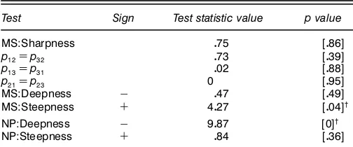
For the later sample period (shown in Table 7), the MS model test continues to reject nonsteepness at the 5% level, in contrast to the NP test, which now ags deepness of recess-sions rather than steepness of expanrecess-sions. The major change in inference using parametric tests is that there is no evidence of sharpness in the later period.
Table 7. Tests for Asymmetries Using the MSIH(3)-AR(4) Model of U.S. Output Growth, 1960:2–1996:2
Test Sign Test statistic value pvalue
MS:Sharpness 075 [086]
p12Dp32 073 [039]
p13Dp31 002 [088]
p21Dp23 0 [095]
MS:Deepness ƒ 047 [049]
MS:Steepness C 4027 [004]†
NP:Deepness ƒ 9087 [0]†
NP:Steepness C 084 [036]
NOTE: The NP and MS test statistics are2(1)under the null of symmetry. A positive
(neg-ative) value of “Sign” ‘ags positive (neg(neg-ative) skewness. üSigni’cance at the 10% level.
†Signi’cance at the 5% level.
6.3 Models of U.S. Investment
and Consumption Growth
To further illustrate the method of testing for asymmetries, we apply the tests to U.S. investment and consumption growth using a number of MS models. These models contain either two or three regimes and either allow the error variance to depend on the regime or restrict it to be heteroscedastic. In all cases we consider models without lags, so that MSI and MSM models are equivalent.
The rst four panels of Figure 4 depict the recession regime probabilities for investment growth. The allocation of obser-vations to the recession regime is more dependent on whether or not the errors are allowed to be heteroscadastic than on whether there are two or three regimes. The main difference between the two- and three-regime models with heteroscedas-tic errors is that there is some evidence of a recession in the investment series around 1990 in the former. Table 8 shows that the model-based steepness tests (MS nonsteepness) reject the null at the 5% level in both the homoscedastic and het-eroscedastic three-regime models and indicate steepness of expansions, whereas the NP tests suggest “tallness” of expan-sions.
The last four panels in Figure 4 give the recession probabil-ities for consumption growth. Here the estimates of the “reces-sion” regime for the two- and three-regime heteroscedastic models are quite different, and from Table 8 the homoscedas-tic model indicates tallness and steepness of expansions, in line with the NP tests, whereas both features are absent in the heteroscedastic model.
These examples suggest a number of points. The results of testing for asymmetries based on parametric models may be sensitive to the model specication used. Specically, it is likely to matter whether the model allows for heteroscedastic errors. The ndings here conrm the Monte Carlo results in Section 5.2. The regime categorization in models that allow heteroscedastic disturbances will reect shifts in both the mean and the variance of the series, and so will not necessar-ily coincide with that in homoscedastic models if, for exam-ple, the shifts in mean and variance are not in line. Thus it is important to adequately capture the business cycle features of the series; we argued in Section 6.2, following Sichel (1994), that for modeling U.S. output growth, a three-regime model with heteroscedastic errors appears to be required. In the case of the investment and consumption series, a closer examina-tion of the individual models would reveal which one is the most appropriate; the results in Table 8 are simply illustrative.
7. CONCLUSIONS
We have set out the parametric restrictions on MS-AR mod-els for the series generated by those modmod-els to exhibit neither deepness, steepness, nor sharpness business cycle asymme-tries. For the popular two-state model rst proposed by Hamil-ton (1989), we have shown that deepness implies sharpness and vice versa, and that the model (at least with Gaussian dis-turbances) cannot generate steepness. For three-state models, which arguably afford a better characterization of the busi-ness cycle, the three concepts are distinct. We showed how
1960 1970 1980 1990 2000 0.5
1.0 MSI(2)AR(0) of DI
1960 1970 1980 1990 2000 0.5
1.0 MSIH(2)AR(0) of DI
1960 1970 1980 1990 2000 0.5
1.0 MSI(3)AR(0) of DI
1960 1970 1980 1990 2000 0.5
1.0 MSIH(3)AR(0) of DI
1960 1970 1980 1990 2000 0.5
1.0 MSI(2)AR(0) of DC
1960 1970 1980 1990 2000 0.5
1.0 MSIH(2)AR(0) of DC
1960 1970 1980 1990 2000 0.5
1.0 MSI(3)AR(0) of DC
1960 1970 1980 1990 2000 0.5
1.0 MSIH(3)AR(0) of DC
Figure 4. MS Models of U.S. Investment and Consumption Growth. Shown are the estimated smoothed probabilities with which each obser-vation falls in the recession regime for a variety of models, for investment growth (top two rows) and consumption growth (bottom two rows).
Table 8. Tests for Asymmetries Using MS-AR Models of U.S. Investment and Consumption Growth
Investment Consumption
MSM(2)
MS:Sharpness 002[089] 7067[001]ü MS:Deepness 3068[006] 4025[004]† MS:Steepness
MSMH(2)
MS:Sharpness 2018[014] 026[061] MS:Deepness 012[073] 032[057] MS:Steepness
MSM(3)
MS:Sharpness 1057[067] 3083[028] p12Dp32 033[056] 003[086]
p13Dp31 1013[029] 3009[008] p21Dp23 015[070] 074[039]
MS:Deepness 079[037] 6079[001]ü MS:Steepness 7061[001]ü 9015[0]ü
MSMH(3)
MS:Sharpness 1004[079] 1073[063] p12Dp32 1001[032] 012[073]
p13Dp31 001[094] 1069[019] p21Dp23 001[093] 0 [094]
MS Nondeepness 1035[025] 013[071] MS Nonsteepness 4077[0029]† 044[051]
Nonparametric tests
NP:Deepness 14032[0]ü 19019[0]ü NP:Steepness 013[072] 7020[001]ü
NOTE: The data are from the FRED database (http://www.stls.frb.org/ fred/data/gdp.html) and cover the period 1960:4–1999:2. Investment growth is the ’rst difference of the log of invest-ment (FRED database mnemonic GPDIC92), and consumption growth is the ’rst difference of the logarithm of consumers’ expenditure (mnemonic PCEDGC92).
üSigni’cant at the 1% level †Signi’cant at the 5% level
the parameter restrictions can be applied as Wald tests, and to illustrate, reported the results of testing for asymmetries in Hamilton’s original model of U.S. output growth and in two-and three-state models of U.S. investment two-and consumption growth. The tests detect rst-moment asymmetries and are not affected by regime-dependent heteroscedasticity, provided that this is modeled.
A comparison of the empirical results for our tests with the NP outcomes suggests that our tests have reasonable power to detect asymmetries. This was conrmed by a Monte Carlo study showing that our tests have good size and power prop-erties and perform well relative to the NP tests. The latter are adversely affected by regime-dependent heteroscedasticity and can give misleading inferences concerning rst-moment asymmetries. Moreover, our tests work reasonably well when the data are generated from other classes of regime-switching models.
ACKNOWLEDGMENTS
Financial support from the U.K. Economic and Social Research Council under grant L138251009 is gratefully acknowledged by both authors. All the computations reported herein were carried with the MSVAR class for Ox: (see Krolzig 1998). Helpful comments were received from two anonymous referees, as well as seminar audiences at the Bank of England, Cambridge, the 1999 Society of Eco-nomic Dynamics Conference at CRENOS, Sardinia, the 1999 Meeting of the European Economic Association, Santiago de Compostela, Exeter University, and Nufeld College. Com-ments from David Hendry and Neil Shephard were especially helpful.