Full Terms & Conditions of access and use can be found at
http://www.tandfonline.com/action/journalInformation?journalCode=ubes20
Download by: [Universitas Maritim Raja Ali Haji] Date: 11 January 2016, At: 19:54
Journal of Business & Economic Statistics
ISSN: 0735-0015 (Print) 1537-2707 (Online) Journal homepage: http://www.tandfonline.com/loi/ubes20
Inference for Time Series Regression Models With
Weakly Dependent and Heteroscedastic Errors
Yeonwoo Rho & Xiaofeng Shao
To cite this article: Yeonwoo Rho & Xiaofeng Shao (2015) Inference for Time Series Regression Models With Weakly Dependent and Heteroscedastic Errors, Journal of Business & Economic Statistics, 33:3, 444-457, DOI: 10.1080/07350015.2014.962698
To link to this article: http://dx.doi.org/10.1080/07350015.2014.962698
View supplementary material
Accepted author version posted online: 25 Sep 2014.
Submit your article to this journal
Article views: 208
View related articles
Inference for Time Series Regression Models
With Weakly Dependent and Heteroscedastic
Errors
Yeonwoo R
HODepartment of Mathematical Sciences, Michigan Technological University, Houghton, MI 49931 ([email protected])
Xiaofeng S
HAODepartment of Statistics, University of Illinois at Urbana-Champaign, Champaign, IL 61820 ([email protected])
Motivated by the need to assess the significance of the trend in some macroeconomic series, this article considers inference of a parameter in parametric trend functions when the errors exhibit certain degrees of nonstationarity with changing unconditional variances. We adopt the recently developed self-normalized approach to avoid the difficulty involved in the estimation of the asymptotic variance of the ordinary least-square estimator. The limiting distribution of the self-normalized quantity is nonpivotal but can be consistently approximated by using the wild bootstrap, which is not consistent in general without studentization. Numerical simulation demonstrates favorable coverage properties of the proposed method in comparison with alternative ones. The U.S. nominal wages series is analyzed to illustrate the finite sample performance. Some technical details are included in the online supplemental material.
KEY WORDS: Heteroscedasticity; Modulated stationary process; Self-normalization; Time series re-gression; Wild bootstrap.
1. INTRODUCTION
Consider the simple linear trend model,
Xt,n=b1+b2(t /n)+ut,n, t=1, . . . , n. (1) Inference of the linear trend coefficientb2is an important
prob-lem in many fields such as econometrics, statistics, and en-vironmental sciences, and there is a rich literature. Hamilton (1994, chap. 16) derived the limiting distribution of the ordinary least-square (OLS) estimators ofb1 andb2when the errors are
independent and identically distributed (iid) from a normal dis-tribution. To account for possible dependence in the error,{ut,n} has often been assumed to be a stationary weakly dependent process. For example, Sherman (1997) applied the subsampling approach when the errors are from a stationary mixing process, and Zhou and Shao (2013) considered theM-estimation with stationary errors whose weak dependence was characterized by physical dependence measures (Wu2005). Another popular way in econometrics is to model the dependence in the error as an au-toregressive (AR) process, and testing procedures that are robust to serial correlation with possible unit root have been developed; see Canjels and Watson (1997), Vogelsang (1998), Bunzel and Vogelsang (2005), and Harvey, Leybourne, and Taylor (2007), among others.
However, there is increasing evidence that many macroe-conomic series exhibit heteroscedastic behavior. For exam-ple, the U.S. gross domestic product series has been observed to have less variability since 1980s; see Kim and Nelson (1999), McConnell and Perez-Quiros (2000), Busetti and Tay-lor (2003), and references therein. In addition, Sensier and van Dijk (2004) argued that majority of the macroeconomic data in Stock and Watson (1999) had abrupt changes in unconditional variances. The empirical evidence of weakly dependent and
heteroscedastic errors can also be found from environmental time series; see Rao (2004), Zhou and Wu (2009), and Zhang and Wu (2011) for their data illustrations using global tempera-ture series. There have been a number of articles on the inference of weakly dependent time series models with heteroscedastic er-rors. For example, Xu and Phillips (2008) studied the inference on the AR coefficients when the innovations are heteroscedas-tic martingale differences. Xu (2008) focused on inference of polynomial trends with errors exhibiting nonstationary volatil-ity. Zhao (2011) and Zhao and Li (2013) explored inferences on the constant mean in the presence of modulated stationary errors. Xu (2012) presented a statistic with a pivotal limiting distribution for the multivariate trend model when the error process is generated from a stationary vector AR process with heteroscedastic innovations.
Our framework generalizes the model (1) in two nontrivial aspects. For one, our trend function is a finite linear combina-tion of deterministic trends, each of which can contain finite number of breaks at known points. Most studies in the literature are restricted to the linear or polynomial trend, but allowing for break in intercept can be useful in practice. For example, if
Xt,n=b1+b21(t > tB)+b3(t /n)+ut,n, that is, a linear trend model with a jump at a known intervention timetB, then testing the significance ofb2is of interest in assessing the significance
of the jump at the intervention in the presence of a linear trend. This kind of one break model was considered in the analysis of nominal wage series by Perron (1989), and its inference is reinvestigated in Section5. For the other, we allow two types of nonstationary processes for the errorsut,n. One type of
non-© 2015American Statistical Association Journal of Business & Economic Statistics July 2015, Vol. 33, No. 3 DOI:10.1080/07350015.2014.962698
444
stationary process is adapted from Cavaliere and Taylor (2007, 2008a, 2008b) and Xu and Phillips (2008). For this class of models, the error process is represented as a linear process of independent but heteroscedastic innovations. This includes au-toregressive moving average (ARMA) models with independent but heteroscedastic innovations as a special case. The other type of nonstationary process is the modulated stationary processes (Zhao2011; Zhao and Li2013), where a stationary process is amplified by a (possibly periodic) deterministic function that only depends on the relative location of an observation. The latter is a type of locally stationary processes (Priestley1965; Dahlhaus1997), as pointed out in Zhao and Li (2013). Together, they cover a wide class of nonstationary but weakly dependent models with unconditional heteroscedasticity.
When the errors are nonstationary with unconditional het-eroscedasticity, the difficulty rises due to the complex form of the asymptotic variance of the OLS estimator. In this article, we apply the wild bootstrap (WB) (Wu1986) to approximate the limiting behavior of the OLS estimator. However, simply applying the wild bootstrap to the unstudentized OLS estimator does not work because it cannot properly capture the terms in the asymptotic variance that are due to temporal dependence in the error. To overcome this difficulty, we propose to adopt the self-normalized (SN) method (Lobato2001; Shao 2010), which was mainly developed for stationary time series. Due to the heteroscedasticity and the nonconstant regressor, the limit-ing distribution of the SN-based quantity is nonpivotal, unlike the existing SN-based methods. The advantage of using the SN method, though, is that the limiting distribution of the studen-tized OLS estimator only depends on the unknown heteroscedas-ticity, which can be captured by the wild bootstrap. Compared to the conventional heteroscedasticity and autocorrelation consis-tent (HAC) method or block-based bootstrap methods that are known to handle mildly nonstationary errors, the use of the SN method and the wild bootstrap are practically convenient and are shown to lead to more accurate inference.
To summarize, we provide an inference procedure of trends in time series that is robust to smooth and abrupt changes in un-conditional variances of the temporally dependent error process, in a quite general framework. Our assumptions on determinis-tic trends and weakly dependent heteroscedasdeterminis-tic errors are less restrictive than those from most earlier works in the trend assess-ment literature. Besides, our inference procedure is convenient to implement. Although our method is not entirely bandwidth-free, the finite-sample performance is not overly sensitive to the choice of the trimming parameterǫ, and its choice is accounted for in the first-order limiting distribution and the bootstrap ap-proximation. The work can be regarded as the first extension of the SN method to the regression model with weakly dependent and heteroscedastic errors. One of the key theoretical contri-butions of the present article is to derive the functional central limit theorem of the recursive OLS estimator, which leads to the weak convergence of the SN-based quantity. At a methodologi-cal level, the self-normalization coupled with the wild bootstrap eliminates the need to directly estimate the temporal depen-dence in the error process. Although some earlier works such as Cavaliere and Taylor (2008b) and Zhao and Li (2013) applied the wild bootstrap for similar error processes, it seems that they need to involve the choice of a block size or consistent
estima-tion of a nuisance parameter to make the wild bootstrap work. In our simulation, our method is demonstrated to deliver more accurate finite-sample coverage compared to alternative meth-ods, and thus inherits a key property of the SN approach that was known to hold only for stationary time series (Shao2010). Recently, Zhou and Shao (2013) extended the SN method to the regression setting with fixed parametric regressors, where the error is stationary and the response variable is only non-stationary in mean. The framework here is considerably more general in that the error is allowed to exhibit local stationarity or unconditional heteroscedasticity and the response variable is nonstationary at all orders. On the other hand, we only consider the inference based on the ordinary least-square (OLS) estima-tor, whereas theM-estimation was considered in Zhou and Shao (2013).
The rest of the article is organized as follows. Section 2 presents the model, the OLS estimation, and the limiting dis-tribution of the OLS estimator. Section3contains a functional central limit theorem for the recursive OLS estimators, which leads to the limiting distribution of the SN-based quantity. The wild bootstrap is described and its consistency for the SN quan-tity is justified in Section3. Section4presents some simulation results and Section5contains an application of our method to the U.S. nominal wage data. Section 6 concludes. Technical details are relegated to a supplemental online appendix.
Throughout the article, we use−→D for convergence in distri-bution and⇒weak convergence inD[ǫ,1] for someǫ∈(0,1), the space of functions on [ǫ,1], which are right continuous and have left limits, endowed with Skorohod metric (Billingsley 1968). The symbols Op(1) and op(1) signify being bounded in probability and convergence to zero in probability, respec-tively. If Op(1) and op(1) are used for matrices, they mean elementwise boundedness and convergence to zero in proba-bility. We use ⌊a⌋to denote the integer part ofa∈R,B(·) a standard Brownian motion, andN(μ, ) the (multivariate) nor-mal distribution with meanμand covariance matrix. Denote by||X||p =(E|X|p)1/p. For ap×q matrixA=(aij)i≤p,j≤q,
where Xt,n is a univariate time series, n is the sample size, β =(b1, . . . , bp)′ is the parameter of interest, and the regres-sors Ft,n= {f1(t /n), . . . , fp(t /n)}′ are nonrandom. The re-gressors{fj(t /n)}
p
j=1are rescaled, thus increasing the sample
size n means we have more data in a local window. We use
F(s)= {f1(s), . . . , fp(s)}′, s∈[0,1] to denote the regressors with relative location s, and we observe Ft,n=F(t /n). Let N =n−p+1, wherepis fixed.
The error process{ut,n}is assumed to be either one of the followings:
(A1)Generalized Linear Process. The error process is defined andLis the lag operator. We further assume
(i) Let ω(s)=limn→∞ω⌊ns⌋,n be some deterministic, positive (cadlag) function ons∈[0,1]. Letω(s) be piecewise Lipschitz continuous with at most finite number of breaks. Ift <0, letωt,n< ω∗ for some 0< ω∗ <∞.
(ii) 0<|C(1)|<∞,j∞=0j|cj|<∞. (iii) E|et|4<∞.
(A2)Modulated Stationary Process.The error process is de-fined as
ut,n=νt,nηt,
where{ηt}is a mean zero strictly stationary process that can be expressed asηt =G(Ft) for some measurable function
GandFt =(. . . , ǫt−1, ǫt), whereǫtare iid (0,1). We further assume
(i) Let ν(s)=limn→∞ν⌊ns⌋,n be some deterministic, positive (cadlag) function ons∈[0,1]. Letν(s) be piecewise Lipschitz continuous with at most finite number of breaks.
The key feature of the two settings above is that they allow both smooth and abrupt changes in the unconditional variance and second-order properties of ut,n through ω(s) in (A1) (i) andν(s) in (A2) (i), which depend only on the relative location
s=t /nin a deterministic fashion. If this part should be con-stant, then the two models correspond to the popular stationary models; the linear process for (A1) and stationary causal pro-cess (Wu2005) for (A2). The model (A1) is considered in, for example, Cavaliere (2005), Cavaliere and Taylor (2007,2008a, 2008b), and Xu and Phillips (2008). The assumptions (A1) (ii) is popular in the linear process literature to ensure the central limit theorem and the invariance principle, and (A1) (iii) implies the existence of the fourth moment of{ut,n}. The model (A2) is adapted from Zhao (2011) and Zhao and Li (2013) and is called the modulated stationary process, which was originally developed to account for the seasonal change, or periodicity, observed in financial or environmental data. The condition (A2) (ii) is slightly stronger than the existence of the fourth mo-ment, which is required in the proof of the bootstrap consis-tency. (A2) (iii) implies that{ut,n}is short-range dependent and the dependence decays exponentially fast. These two classes of models are both nonstationary and nonparametric, which
represent extensions of stationary linear/nonlinear processes to nonstationary weakly dependent processes with unconditional heteroscedasticity.
Remark 2.1. Note that the model (A1) is a special case of Xu and Phillips (2008), but it can be made as general as the framework of Xu and Phillips (2008), by lettingetbe a martin-gale difference sequence with its natural filtrationEtsatisfying n−1nt=1E(et2|Et−1)→C <∞for some positive constantC, rather than an iid sequence. See Remark 1 of Cavaliere and Tay-lor (2008b). In this article, we do not pursue this generalization only for the simplicity in the proofs. For (A2), our framework for the modulation,ν(s) is more general than that of Zhao (2011). For example, the so-called “k-block asymptotically equal cumu-lative variance condition” in Definition 1 in Zhao (2011) rules out a linear trend in the unconditional variance. The model (A2) can be replaced with some mixing conditions for the stationary part, but the details are omitted for simplicity. It is worthwhile to stress that both (A1) and (A2) are based on already popular and widely used stationary models, and they extend those stationary models by incorporating heteroscedasticity in a natural way.
In this article, we are interested in the inference of β =(b1, . . . , bp)′, based on the OLS estimator βN = (nt=1Ft,nFt,n′ )
−1
(nt=1Ft,nXt,n). If the errors satisfy (A1) or (A2) and the fixed regressorsF(s) are piecewise Lipschitz con-tinuous, then under certain regularity conditions, the OLS esti-mator is approximately normally distributed, that is,
n1/2(βN−β)
D
−→N(0p, ), (2) where the covariance matrix has the sandwich form
Q−11V Q−11,Q1=
The statement (2) is a direct consequence of Theorem 3.1. No-tice thatQ1can be consistently estimated byn−1
n
t=1Ft,nFt,n′ , but V depends on the nuisance parameters C(1), Ŵ, and
{ω(s), ν(s);s∈[0,1]}. To perform hypothesis testing or con-struct a confidence region forβ, the conventional approach is to consistently estimate the unknown matrixV using, for ex-ample, the HAC estimator in Andrews (1991). The HAC es-timator involves a bandwidth parameter, and the finite sample performance critically depends on the choice of this bandwidth parameter. Moreover, the consistency of the HAC estimator is shown under the assumption that the errors are stationary or ap-proximately stationary (Newey and West1987; Andrews1991). Alternatively, block-based resampling approaches (Lahiri2003) such as the moving block bootstrap and subsampling (Politis, Romano, and Wolf1999) are quite popular to deal with the de-pendence in the error process, see Fitzenberger (1998), Sherman (1997), and Romano and Wolf (2006) among others. However, these methods are designed for stationary processes with differ-ent blocks having the same or approximately the same stochastic property. Note that Paparoditis and Politis (2002) proposed the so-called local block bootstrap for the inference of the mean with locally stationary errors. Their method involves two tuning parameters and no guidance on their choice seems provided.
There have been recently proposed alternative methods to the HAC-based inference for dynamic linear regression models such as Kiefer, Vogelsang, and Bunzel (2000; KVB, hereafter). KVB’s approach is closely related to the SN method by Lobato (2001) and Shao (2010). The KVB and SN methods share the same idea that by using an inconsistent estimator of asymp-totic variance, a bandwidth parameter can be avoided. In finite samples this strategy is shown to achieve better coverage and size compared to the conventional HAC-based inference. In a recent article by Rho and Shao (2013), the KVB method is shown to differ from the SN method in the regression setting: the KVB method applies an inconsistent recursive estimation of the “meat” partVof the covariance matrixin (2) and consis-tently estimates the “bread” partQ1, whereas the SN method
involves the inconsistent recursive estimation for the whole co-variance matrix. Although the KVB and SN methods have the same limiting distribution, Rho and Shao (2013) had shown in their simulations that the SN method tends to have better finite sample performance than the KVB method. For this reason, we adopt the SN method for our problem.
To apply the SN method, we need to define an inconsistent estimate ofbased upon recursive estimates ofβ. Consider the OLS estimatorβt =βt,N ofβ using the firstt+p−1 obser-(0,1) is a trimming parameter. Define the SN quantity
TN =N major role of this self-normalizer is to remove nuisance parame-ters in the limiting distribution of the SN quantityTN, rather than as a consistent estimator of the true asymptotic variance. With stationary errors, the same self-normalizer does this job well, providing pivotal limiting distributions for TN. However, un-der our framework of nonstationary errors, the self-normalizer
N(ǫ) cannot completely get rid of the nuisance parameter in the limiting distribution ofTN, as seen from the next section.
3. INFERENCE
For the regressorFt,n, we impose the following assumptions.
(R1) For allr∈[ǫ,1],Qr =r−1 tinuous with at most finite number of breaks.
The assumptions (R1) and (R2) are satisfied by commonly used trend functions such as fj(s)=sτ for some nonnega-tive integerτ,fj(s)=sin(2π s) or cos(2π s). The assumption infr∈[ǫ,1]det(Qr)>0 in (R1) excludes the collinearity of fixed regressors and is basically equivalent to the assumption (C4) in Zhou and Shao (2013), and the trimming parameterǫ∈(0,1) has to be chosen appropriately. The assumption (R1) appears slightly weaker than Kiefer, Vogelsang, and Bunzel’s (2000)
Assumption 2, ⌊nr⌋−1⌊t=nr1⌋Ft,nFt,n′ =Q+op(1) for some p×pmatrixQ, which is identical for allr∈(0,1]. Although, in general, Kiefer, Vogelsang, and Bunzel (2000) allowed for dynamic stationary regressors whereas our framework targets fixed regressors, our method can be extended to allow for dy-namic regressors by conditioning on the regressors. Since our work is motivated by the trend assessment of macroeconomic series, it seems natural to assume the regressor is fixed. The assumption (R2) allows for structural breaks in trend functions.
Theorem 3.1. Assume (R1)–(R2).
(i) Let the error process{ut,n}be generated from (A1). The recursive OLS estimator β⌊N r⌋ of β converges weakly, that is,
Remark 3.1. For a technical reason, the above functional cen-tral limit theorem has been proved onD[ǫ,1] for someǫ∈(0,1) instead of onD[0,1]. For most of the trend functions that include polynomialsτwithτ >1/2 or sin(2π s), thisǫhas to be strictly greater than 0. However, for some trend functions,ǫcan be set as 0. In particular, when the trend function is a constant mean func-tion, thenQr =1 forr∈(0,1],BF(r)=
In any case, the choice of trimming parameter ǫ is captured by the first-order limiting distribution in the same spirit of the fixed-bapproach (Kiefer and Vogelsang2005).
Remark 3.2. If the trend function has breaks, the trim-ming parameter ǫ has to be rather carefully chosen so that the condition (R1) can be satisfied. For example, if we use a linear trend function with a jump in the mean, that is,
Xt,n=b1+b21(t > tB)+b3(t /n)+ut,n, with a break point at the choice of trimming parameter does not seem to affect the finite sample performance much, as we can see in the simulation reported in Section4.3.
The limiting distributionLFin Theorem 3.1 is not pivotal due to the heteroscedasticity of the error process and nonconstant nature ofQr. If the error process is stationary, thenω(s)≡ω in (A1) andν(s)≡ν in (A2) would be canceled out, and the only unknown part in the limiting distribution isQr. IfQr =Q, r∈[ǫ,1] for somep×pmatrixQ, thenQwould be canceled
out in the limiting distribution, which occurs in the use of the SN method for stationary time series with a constant regressor; see Lobato (2001) and Shao (2010). In our case, the part that reflects the contribution from the temporal dependence, C(1) orŴ, does cancel out. However, the heteroscedasticity remains even ifQr =Q, and the limiting distribution still depends on the unknown nuisance parameter{ω(s), ν(s);s∈[0,1]}.
Estimating unknown parameters inLFseems quite challeng-ing due to the estimation of ω(s),ν(s), and integral of them over a Brownian motion. Instead of directly estimating the un-known parameters, we approximate the limiting distributionLF using the wild bootstrap introduced in Wu (1986). Although there has been some recent attempts to use the wild bootstrap to the trend assessment with nonstationary errors (e.g., Xu (2012) for the linear trend model and Zhao and Li (2013) for the con-stant mean model), this article seems to be the first to apply the wild bootstrap to the SN-based quantity. The main reason the wild bootstrap works for the SN method in such settings is that the part due to the temporal dependence, which is difficult to capture with the wild bootstrap, no longer exist in the limiting distribution LF of the SN-based quantity so that LF can be consistently approximated by the wild bootstrap. In contrast, without the self-normalization, the unknown nuisance parame-terC(1) orŴstill remains in the limiting distribution, and thus, the wild bootstrap is not consistent in this case.
Letut,n=Xt,n−Ft,n′ βN denote the residuals. We first gen-erate the resampled residualsu∗
t,n=ut,nWt, whereWt is a se-quence of external variables. Then we generate the bootstrap responses as Xn, andLF can be approximated by its bootstrap counterpart. We assume
distribution with mean zero or use the distribution recommended by Mammen (1993). Notice that there are no user-determined parameters, which makes the wild bootstrap convenient to im-plement in practice.
t=1. The following theorem states
the consistency of the wild bootstrap.
Theorem 3.2. Assume (R1)–(R2) and (B1).
(i) If{ut,n}is generated from (A1), we have
(iii) It follows from the continuous mapping theorem that
TN∗ =N(βN∗ −βN)′{∗N(ǫ)}
andLF as defined in Theorem 3.1.
Remark 3.3. Notice that the wild bootstrap cannot success-fully replicate the original distribution without the normaliza-tion, unless C2
(1)=D(1) or Ŵ=1, because the wild boot-strap cannot capture the temporal dependence of the original error series. However, in the limiting distribution of
N−1/2⌊N r⌋(β
⌊N r⌋−β), the part that reflects the long run de-pendence,C(1) orŴ, can be separated from the rest, for both data-generating processes (A1) and (A2). This property makes it possible to construct a self-normalized quantity, whose limiting distribution depends only on the heteroscedastic part (captured by the wild bootstrap), not on the temporal dependence part.
Remark 3.4. Hypothesis testing can be conducted following the argument in Zhou and Shao (2013). Let the null hypothesis beH0:Rβ=λ, whereRis ak×p(k≤p) matrix with rankk test can be formed by using the bootstrapped critical values, owing to the fact that in probability under the assumptions of Theorem 3.2. For exam-ple, if we letk=1,λ=0, andRbe a vector of 0’s except for the jth element being 1, we can construct a confidence interval or test the significance of individual regression coefficientbj. Letβt,j be thejth element ofβt. The 100(1−α)% confidence interval the jth element of the OLS estimate of β using theith boot-strapped sample, andBis the number of bootstrap replications.
Remark 3.5. Our method is developed in the same spirit of Xu (2012), who focused on the multivariate trend inference under the assumption that the trend is linear and errors follow a VAR(p) model with heteroscedastic innovations. In particular, Xu’s Class 4 test used the studentizer first proposed in Kiefer, Vogelsang, and Bunzel (2000) and the wild bootstrap to capture the heteroscedasticity in the innovations. Since the KVB method and the SN method are closely related (see Rho and Shao2013 for a detailed comparison), it seems that there are some overlap between our work and Xu (2012). However, our work differs from Xu’s in at least three important aspects.
1. The settings in these two articles are different. Xu (2012) allowed for multivariate time series and is interested in the
inference of linear trends, whereas ours is restricted to uni-variate time series. Our assumption on the form of the trend function and the error structure are considerably more gen-eral. In particular, we allow for more complex trend functions as long as it is known up to a finite-dimensional parameter. In addition, the AR(p) model with heteroscedastic innova-tion used by Xu (2012) is a special case of our (A1), that is, linear process with heteroscedastic innovations. Also Xu’s method does not seem directly applicable to the modulated stationary process (A2) we assumed for the errors.
2. The wild bootstrap is applied to different residuals. In Xu’s work, he assumed VAR(p) structure for the error process with known p. He needs to estimate the VAR(p) model to obtain the residuals, which are approximately independent but heteroscedastic. His wild bootstrap is applied to the resid-uals from the VAR(p) model, and is expected to work due to the well-known ability of wild bootstrap to capture het-eroscedasticity. By contrast, we apply the wild bootstrap to OLS residuals from the regression model and our OLS residuals are both heteroscedastic and temporally dependent. The wild bootstrap is not expected to capture/mimic tempo-ral dependence, but since the part that is due to tempotempo-ral dependence is cancelled out in the limiting distribution of our self-normalized quantity, the wild bootstrap successfully captures the remaining heteroscedasticity and provides a con-sistent approximation of the limiting distribution. Note that our method works for errors of both types, but it seems that Xu’s method would not work for the modulated stationary process as assumed in (A2) without a nontrivial modification. 3. Xu’s Class 4 test without prewhitening is in a sense an ex-tension of Kiefer, Vogelsang, and Bunzel (2000) to the linear trend model, whereas our method is regarded as an extension of SN method to the regression setting. In time series regres-sion framework, Rho and Shao (2013) showed that there is a difference between the SN method and the KVB method; see Remark 3.1 therein and also Section2for a detailed ex-planation. It is indeed possible to follow the KVB method in our framework and we would expect the wild bootstrap to be consistent to approximate the limiting distribution of the studentized quantity owing to the separable structure of the errors. To save space, we do not present the details for the KVB studentizer in our setting. Finite sample com-parison between our method and Xu’s Class 3 and 4 tests are provided in Section4.2.
4. SIMULATIONS
In this section, we compare the finite sample performance of our method to other comparable methods in Zhao (2011) and Xu (2012) for (i) constant mean models, (ii) linear trend models, and (iii) linear trend models with a break in the intercept. For the constant mean models, Zhao’s method is applicable only when the errors have periodic heteroscedasticity. On the other hand, Xu’s method can be used only for the linear trend models when the errors are from an AR process. In the cases where neither Zhao’s nor Xu’s methods can be directly applied, we compare our method to the conventional HAC method. Although it has not been rigorously proven that the traditional HAC method works in our framework, we can construct a HAC-type estimator
that consistently estimatesVin (2). Define
Vn,ln can be shown to be consistent for appropriately chosenln, and the inference is based on
TNHAC=n in the linear trend testing context, this statistic is almost identical to the Class 3 test without prewhitening in Xu (2012).
4.1 Constant Mean Models
Consider the linear model
Xt,n=μ+ut,n, t=1, . . . , n, (5) whereμis an unknown constant. Without loss of generality, let
μ=0. Note that for this constant mean models our method is completely bandwidth free, since the trimming parameter can be set to be 0, as mentioned in Remark 3.1.
We conduct two sets of simulations for different kinds of er-ror processes. The first simulation follows the data-generating process in Zhao (2011), where the error process{ut,n}is mod-ulated stationary and has periodic heteroscedasticity. Consider the model (A2) withv(t /n)=cos(3π t /n) and
(M1)ηt =ξt−E(ξt),ξt=θ|ξt−1| +(1−θ2) 1/2
ǫt,|θ|<1, (M2)ηt =∞j=0ajǫt−j, aj =(j+1)−ζ/10, ζ >1/2, whereǫt are independent standard normal variables in M1. We consider M2 with two different kinds of innovations: M2-1 de-notes M2 with standard normal innovations, and M2-2 stands for M2 witht-distributed innovations withk=3,4,5 degrees of freedom. We used 10,000 replications to get the coverage and interval length with nominal level 95% and sample size
n=150. In each replication, 1000 pseudoseries of iidN(0,1)
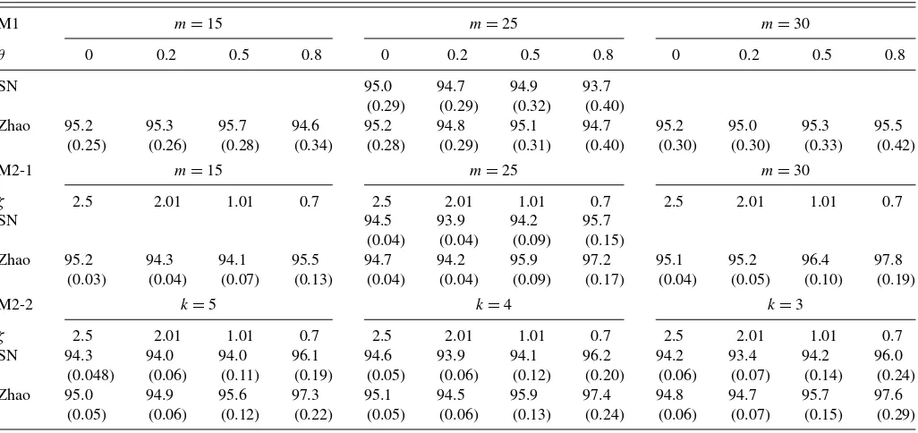
Wt are generated. The coverage rates and interval lengths of Zhao’s method (Zhao) and our method (SN) are reported in Table 1. Note that our method does not require any user-chosen number in this particular example and min the table is only for Zhao’s method. With our choice ofv(t /n), Zhao’s “k-block asymptotically equal cumulative variance condition” holds form=25,50,75, . . ., which means that whenm=15 and 30 in M1 and M2-1, the conditions in Zhao (2011) are not satisfied. For the model M2-2,m=25 is used for Zhao’s method.
Zhao (2011) provided a comparison with some existing block-based bootstrap methods and showed that his method tends to have more accurate coverage rates. Our method is comparable to Zhao’s based on our simulation. For the nonlinear thresh-old autoregressive models M1, it seems that our method de-livers slightly less coverage especially when the dependence
Table 1. Percentages of coverage of the 95% confidence intervals (mean lengths of the interval in the parentheses) of the meanμin (5), where μis set to be zero. The error processes are from Zhao’s (2011) setting with periodic heteroscedasticity. The method in Zhao (2011) and our method are compared. The interval lengths of the confidence intervals are in the parentheses. The number of replications is 10,000, and 1000
pseudoseries with iidN(0, 1) are used for the wild bootstrap
M1 m=15 m=25 m=30
θ 0 0.2 0.5 0.8 0 0.2 0.5 0.8 0 0.2 0.5 0.8
SN 95.0 94.7 94.9 93.7
(0.29) (0.29) (0.32) (0.40)
Zhao 95.2 95.3 95.7 94.6 95.2 94.8 95.1 94.7 95.2 95.0 95.3 95.5
(0.25) (0.26) (0.28) (0.34) (0.28) (0.29) (0.31) (0.40) (0.30) (0.30) (0.33) (0.42)
M2-1 m=15 m=25 m=30
ζ 2.5 2.01 1.01 0.7 2.5 2.01 1.01 0.7 2.5 2.01 1.01 0.7
SN 94.5 93.9 94.2 95.7
(0.04) (0.04) (0.09) (0.15)
Zhao 95.2 94.3 94.1 95.5 94.7 94.2 95.9 97.2 95.1 95.2 96.4 97.8
(0.03) (0.04) (0.07) (0.13) (0.04) (0.04) (0.09) (0.17) (0.04) (0.05) (0.10) (0.19)
M2-2 k=5 k=4 k=3
ζ 2.5 2.01 1.01 0.7 2.5 2.01 1.01 0.7 2.5 2.01 1.01 0.7
SN 94.3 94.0 94.0 96.1 94.6 93.9 94.1 96.2 94.2 93.4 94.2 96.0
(0.048) (0.06) (0.11) (0.19) (0.05) (0.06) (0.12) (0.20) (0.06) (0.07) (0.14) (0.24)
Zhao 95.0 94.9 95.6 97.3 95.1 94.5 95.9 97.4 94.8 94.7 95.7 97.6
(0.05) (0.06) (0.12) (0.22) (0.05) (0.06) (0.13) (0.24) (0.06) (0.07) (0.15) (0.29)
is strong and slightly wider confidence intervals compared to Zhao’s method with correctly specifiedm. However, for the lin-ear process models M2, our method has better coverage and slightly narrower intervals whenζis small, that is, when depen-dence is too strong so that the short-range dependepen-dence condition (A2) (iii) does not hold.
In the second simulation, the errorsut,nare generated from (A1) with an AR(1) model. Letetbe generated from iidN(0,1). For (A1),ut,n=ρut−1,n+ω(t /n)et,t =1, . . . , n, which sat-isfies the condition (A1) (ii) and (iii), by lettingcj =ρj. For ω(s), we consider the single volatility shift model
ω2(s)=σ02+(σ12−σ02)1(s≥τ), s ∈[0,1], τ∈(0,1). (6) We let the location of the breakτ ∈ {0.2,0.8}, the initial vari-anceσ02=1, and the ratioδ=σ0/σ1∈ {1/3,3}. This kind of
break model and the choice of parameters were used in Cav-aliere and Taylor (2007, 2008a, 2008b). Here, sample size
n∈ {100,250} and the AR coefficient ρ ∈ {0,0.5,0.8}, and 2000 replications are used to get the coverage percentages and average interval lengths. For the wild bootstrap, {Wt}nt=1 are
generated from iidN(0,1), and we use 1000 bootstrap repli-cations. We also try the two-point distribution in Mammen (1993) for the bootstrap and get similar simulation results (not reported).
Since this error structure do not show any periodicity, Zhao’s method is no longer applicable. We use the HAC-type quantity introduced in (4) to make a comparison with our method. How-ever, the performance of the HAC-based method is sensitive to the user-chosen parameterln, the choice of which is often diffi-cult. For the purpose of our simulation, we choose the oracle op-timalln, favoring the HAC method. Specifically, since we know the true V, we chooseln such that ˆl=argminl||Vn,ln−V||
2
F,
where|| · ||Fstands for the Frobenius norm. Note that this choice oflnis not feasible in practice. For the choice of the kernel, we use the Bartlett kernel, that is,a(s)=(1− |s|)1(|s| ≤1), which guarantees the positive-definiteness ofVn,ln.
The results are presented inTable 2. The columns under the HAC (l) represent the result using the HAC-type quantity with ˆ
l, ˆl/2, and 2ˆl. Whenρ=0, the optimal bandwidths chosen for the HAC estimators arel=1, so we do not have any values for the column corresponding to ˆl/2.
Ifρ =0, all methods perform very well, which is expected because the error process is simply iid with some heteroscedas-ticity. The wild bootstrap without the self-normalization is also consistent becauseC(1)=1. However, as the dependence in-creases, the performance of all methods gets worse. Ifρ=0, the wild bootstrap without the self-normalization is no longer con-sistent and thus produces the worst coverage. Of the three types of methods considered (SN-WB, WB, HAC), the SN method with the wild bootstrap delivers the most accurate coverage probability. For the case of moderate dependenceρ=0.5, the SN-WB method still performs quite well, while the HAC-type method shows some undercoverage. When the temporal depen-dence strengthens, that is, ρ =0.8, the SN-WB method de-livers the best coverage. For the HAC-type method, note that the optimal bandwidth is chosen to minimize the distance from the true covariance matrix. However, this choice of the band-width may not coincide with the bandband-width that produces the best coverage; as can be seen for the cases (τ, δ)=(0.2,3) or (τ, δ)=(0.8,0.33), where 2ˆltends to produce better coverage than ˆl. The interval lengths for the SN-WB method are some-what longer than those of HAC methods, but considering the gain in coverage accuracy, this increase of interval length seems reasonable.
Table 2. Percentages of coverage of the 95% confidence intervals (mean lengths of the interval in the parentheses) of the meanμin (5), where μis set to be zero. The error processes exhibit nonperiodic heteroscedasticity; (A1)–AR(1) with single volatility shift (6). The number of
replications is 2000, and 1000 pseudoseries with iidN(0, 1) are used for the wild bootstrap
Model HAC (l)
n τ δ ρ SN-WB WB lˆ l/2ˆ 2ˆl lˆ
100 0.2 0.33 0 94.5(1.3) 94.5(1.1) 94.8(1.1) — 94.5(1.1) 1
100 0.2 3 0 94.8(0.2) 94.8(0.2) 94.9(0.2) — 94.8(0.2) 1
100 0.8 0.33 0 94.8(0.7) 93.5(0.6) 93.6(0.6) — 93.9(0.6) 1
100 0.8 3 0 94.3(0.4) 94.8(0.4) 95.0(0.4) — 94.5(0.3) 1
250 0.2 0.33 0 95.2(0.8) 94.7(0.7) 94.8(0.7) — 94.8(0.7) 1
250 0.2 3 0 95.0(0.1) 94.8(0.1) 94.8(0.1) — 95.0(0.1) 1
250 0.8 0.33 0 95.0(0.4) 94.9(0.4) 94.9(0.4) — 95.0(0.4) 1
250 0.8 3 0 94.3(0.3) 95.0(0.2) 95.2(0.2) — 94.8(0.2) 1
100 0.2 0.33 0.5 93.2(2.4) 70.8(1.2) 87.5(1.8) 84.5(1.6) 87.4(1.8) 6
100 0.2 3 0.5 94.8(0.5) 73.6(0.2) 89.0(0.3) 83.2(0.3) 90.5(0.4) 5
100 0.8 0.33 0.5 93.7(1.4) 72.5(0.7) 88.8(1.0) 81.7(0.9) 90.0(1.0) 5
100 0.8 3 0.5 93.5(0.8) 71.9(0.4) 88.7(0.6) 85.1(0.5) 88.4(0.6) 6
250 0.2 0.33 0.5 94.7(1.6) 74.2(0.8) 91.6(1.2) 88.7(1.1) 91.5(1.2) 8
250 0.2 3 0.5 95.0(0.3) 73.5(0.2) 91.1(0.2) 86.1(0.2) 92.3(0.2) 6
250 0.8 0.33 0.5 94.3(0.9) 74.0(0.5) 91.6(0.7) 87.6(0.6) 93.3(0.7) 6
250 0.8 3 0.5 93.5(0.5) 73.5(0.3) 91.6(0.4) 89.0(0.4) 91.8(0.4) 8
100 0.2 0.33 0.8 90.8(5.4) 45.1(1.7) 80.5(3.7) 75.1(3.2) 79.1(3.7) 13
100 0.2 3 0.8 92.2(1.1) 45.6(0.3) 82.6(0.7) 74.7(0.6) 84.1(0.8) 11
100 0.8 0.33 0.8 90.8(3.0) 47.9(1.0) 83.8(2.1) 76.0(1.7) 84.2(2.1) 11
100 0.8 3 0.8 89.8(1.9) 45.6(0.6) 80.2(1.3) 75.1(1.1) 79.0(1.3) 13
250 0.2 0.33 0.8 93.2(3.7) 46.9(1.1) 87.3(2.7) 80.8(2.3) 87.9(2.8) 15
250 0.2 3 0.8 93.8(0.7) 48.8(0.2) 87.4(0.5) 80.6(0.4) 90.0(0.5) 15
250 0.8 0.33 0.8 93.0(2.1) 47.7(0.6) 89.3(1.5) 82.0(1.3) 90.5(1.6) 15
250 0.8 3 0.8 92.5(1.3) 47.9(0.4) 87.0(0.9) 80.8(0.8) 87.6(0.9) 15
4.2 Linear Trend Models
In this subsection, we are interested in inference on the linear trend coefficient from a linear trend model
Xt,n=b1+b2(t /n)+ut,n, t=1, . . . , n. (7)
Without loss of generality, letb1=0 andb2=5. The error
pro-cess{ut,n}follows the same setting as in the second simulation of Section4.1, except that{ut,n}is either generated from AR(1) or MA(1), that is,
AR(1) :ut,n=ρut−1,n+εt,n, MA(1) :ut,n=θ εt−1,n+εt,n,
whereεt,n=ω(t /n)et,et iidN(0,1), andω(s) as in (6). For this setting, Xu’s (2012) methods can be used. In fact, Xu’s Class 3 test is almost identical to the HAC-type method in (4). Xu’s Class 4 test is a fixed-bversion of his Class 3 test, and it is closely related to our method, as mentioned in Remark 3.5. For this reason, we compare our method with Xu’s Class 3 and 4 tests. In addition to his original statistics, Xu further applied the prewhitening. In our simulation, we examine finite sample
performance of the following methods:
“SN-WB(ǫ)” Our method with various values for the trimming parameterǫ,
“WB” Wild bootstrap without self-normalization,
“F3” Xu’ s Class 3 test without prewhitening with
χ2limiting distribution,
“PW3” Xu’s prewhitened Class 3 test withχ2
limiting distribution,
“iid” Xu’ s prewhitened Class 3 test with the iid bootstrap,
“WB” Xu’s prewhitened Class 3 test with the wild bootstrap,
“F4” Xu’s Class 4 test without prewhitening with the wild bootstrap,
“PW4” Xu’s prewhitened Class 4 test with the wild bootstrap.
For Xu’s Class 3 tests, we need to choose the truncation parameter. Following Xu, we used Andrews’ (1991) bandwidth selection for AR(1) or MA(1) model with Bartlett kernel. In the implementation of the wild bootstrap for Xu’s method, we assumed the true order of the AR structure of the error process is known.
Remark 4.1. It should be noted that a direct comparison of our method and Xu’s methods is not fair. We gave some advantages
to Xu’s methods in two aspects. The first aspect is that we assume the knowledge of the true error model, VAR(1), following Xu (2012), which may be unrealistic in practice. Xu’s methods can take advantages of this knowledge of the true model; one advantage is that their bootstrap samples are generated following the correctly specified data-generating process, and the other
advantage is that his Class 3 tests can be based on the most (theoretically) efficient choice of the bandwidth parameters. In contrast, our method does not rely on parametric assumption on the error structure, so knowing the true data-generating process does not provide useful information in the implementation of our method. The second aspect is that some of Xu’s methods use
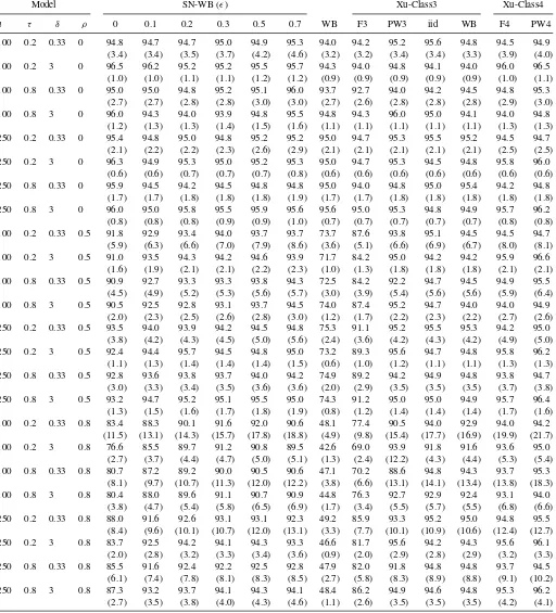
Table 3. Percentages of coverage of the 95% confidence intervals (mean lengths of the interval in the parentheses) of the linear trend model (7) with (b1,b2)=(0, 5), (A1)–AR(1), single volatility shifts. The number of replications is 2000, and 1000 pseudoseries with iidN(0, 1) are used
for the wild bootstrap
Model SN-WB (ǫ) Xu-Class3 Xu-Class4
n τ δ ρ 0 0.1 0.2 0.3 0.5 0.7 WB F3 PW3 iid WB F4 PW4
100 0.2 0.33 0 94.8 94.7 94.7 95.0 94.9 95.3 94.0 94.2 95.2 95.6 94.8 94.5 94.9 (3.4) (3.4) (3.5) (3.7) (4.2) (4.6) (3.2) (3.2) (3.4) (3.4) (3.3) (3.9) (4.0) 100 0.2 3 0 96.5 96.2 95.2 95.2 95.5 95.7 94.3 94.0 94.8 94.1 94.0 96.0 96.5
(1.0) (1.0) (1.1) (1.1) (1.2) (1.2) (0.9) (0.9) (0.9) (0.9) (0.9) (1.0) (1.1) 100 0.8 0.33 0 95.0 95.0 94.8 95.2 95.1 96.0 93.7 92.7 94.0 94.2 94.5 94.8 95.3
(2.7) (2.7) (2.8) (2.8) (3.0) (3.0) (2.7) (2.6) (2.8) (2.8) (2.8) (2.9) (3.0) 100 0.8 3 0 96.0 94.3 94.0 93.9 94.8 95.5 94.8 94.3 96.0 95.0 94.1 94.0 94.8
(1.2) (1.3) (1.3) (1.4) (1.5) (1.6) (1.1) (1.1) (1.1) (1.1) (1.1) (1.3) (1.3) 250 0.2 0.33 0 95.4 94.8 95.0 94.8 95.2 95.2 95.0 94.7 95.3 95.5 95.2 94.5 94.7
(2.1) (2.2) (2.2) (2.3) (2.6) (2.9) (2.1) (2.1) (2.1) (2.1) (2.1) (2.5) (2.5) 250 0.2 3 0 96.3 94.9 95.3 95.0 95.2 95.3 95.0 94.7 95.3 94.5 94.8 95.8 96.0
(0.6) (0.6) (0.7) (0.7) (0.7) (0.8) (0.6) (0.6) (0.6) (0.6) (0.6) (0.6) (0.6) 250 0.8 0.33 0 95.9 94.5 94.2 94.5 94.8 94.8 95.0 94.0 94.8 95.0 95.4 94.2 94.8
(1.7) (1.7) (1.8) (1.8) (1.8) (1.9) (1.7) (1.7) (1.8) (1.8) (1.8) (1.8) (1.8) 250 0.8 3 0 96.0 95.0 95.8 95.5 95.9 95.6 95.6 95.0 95.3 94.8 94.9 95.7 96.2
(0.8) (0.8) (0.8) (0.9) (0.9) (1.0) (0.7) (0.7) (0.7) (0.7) (0.7) (0.8) (0.8) 100 0.2 0.33 0.5 91.8 92.9 93.4 94.0 93.7 93.7 73.7 87.6 93.8 95.1 94.5 94.5 94.7
(5.9) (6.3) (6.6) (7.0) (7.9) (8.6) (3.6) (5.1) (6.6) (6.9) (6.7) (8.0) (8.1) 100 0.2 3 0.5 91.0 93.5 94.3 94.2 94.6 93.9 71.7 84.2 95.0 94.2 94.2 95.9 96.6
(1.6) (1.9) (2.1) (2.1) (2.2) (2.3) (1.0) (1.3) (1.8) (1.8) (1.8) (2.1) (2.1) 100 0.8 0.33 0.5 90.9 92.7 93.3 93.3 93.8 94.3 72.5 84.2 92.2 94.7 94.5 94.9 95.5
(4.5) (4.9) (5.2) (5.3) (5.6) (5.7) (3.0) (3.9) (5.4) (5.6) (5.6) (5.9) (6.4) 100 0.8 3 0.5 90.5 92.5 92.8 93.1 93.7 94.5 74.0 87.4 95.2 94.7 94.0 94.0 94.9
(2.0) (2.3) (2.5) (2.6) (2.8) (3.0) (1.2) (1.7) (2.2) (2.3) (2.2) (2.7) (2.6) 250 0.2 0.33 0.5 93.5 94.0 93.9 94.2 94.5 94.8 75.3 91.1 95.2 95.5 95.3 94.2 95.0
(3.8) (4.2) (4.3) (4.5) (5.0) (5.6) (2.4) (3.6) (4.2) (4.3) (4.2) (4.9) (5.0) 250 0.2 3 0.5 92.4 94.4 95.7 94.5 94.8 95.0 73.2 89.3 95.6 94.7 94.8 95.8 96.2
(1.1) (1.3) (1.4) (1.4) (1.4) (1.5) (0.6) (1.0) (1.2) (1.1) (1.1) (1.3) (1.3) 250 0.8 0.33 0.5 92.8 93.6 93.8 93.7 94.0 94.2 74.9 89.2 94.2 94.9 94.8 93.8 94.7
(3.0) (3.3) (3.4) (3.5) (3.6) (3.6) (2.0) (2.9) (3.5) (3.5) (3.5) (3.7) (3.8) 250 0.8 3 0.5 93.2 94.7 95.2 95.1 95.5 95.0 74.3 91.2 95.0 95.0 94.9 95.7 96.4
(1.3) (1.5) (1.6) (1.7) (1.8) (1.9) (0.8) (1.2) (1.4) (1.4) (1.4) (1.7) (1.6) 100 0.2 0.33 0.8 83.4 88.3 90.1 91.6 92.0 90.6 48.1 77.4 90.5 94.0 92.9 94.0 94.2
(11.5) (13.1) (14.3) (15.7) (17.8) (18.8) (4.9) (9.8) (15.4) (17.7) (16.9) (19.9) (21.7) 100 0.2 3 0.8 76.6 85.5 89.7 91.2 90.8 89.5 42.6 69.0 93.9 91.8 91.6 93.6 95.0
(2.7) (3.7) (4.4) (4.7) (5.0) (5.1) (1.3) (2.4) (12.2) (4.3) (4.4) (5.3) (5.4) 100 0.8 0.33 0.8 80.7 87.2 89.2 90.0 90.5 90.6 47.1 70.2 88.6 94.8 94.3 93.7 95.3
(8.1) (9.7) (10.7) (11.3) (12.0) (12.2) (3.8) (6.6) (13.1) (14.1) (13.4) (13.8) (18.3) 100 0.8 3 0.8 80.4 88.0 89.6 91.1 90.7 90.9 44.8 76.3 92.7 92.9 92.4 93.1 94.0
(3.8) (4.7) (5.4) (5.8) (6.5) (6.9) (1.7) (3.4) (5.5) (5.7) (5.5) (6.8) (6.6) 250 0.2 0.33 0.8 88.0 91.6 92.6 93.1 93.1 92.3 49.2 85.9 93.3 95.2 95.0 94.8 95.5
(8.4) (9.6) (10.1) (10.7) (12.0) (13.1) (3.3) (7.7) (10.1) (10.9) (10.6) (12.4) (12.7) 250 0.2 3 0.8 83.7 92.5 94.2 94.1 94.3 93.3 46.6 81.7 95.6 94.2 94.3 95.6 96.1
(2.0) (2.8) (3.2) (3.3) (3.4) (3.6) (0.9) (2.0) (2.9) (2.8) (2.9) (3.2) (3.3) 250 0.8 0.33 0.8 85.5 91.6 92.4 92.2 92.5 92.8 47.9 82.0 91.8 94.8 94.8 93.7 94.5
(6.1) (7.4) (7.8) (8.1) (8.3) (8.5) (2.7) (5.8) (8.3) (8.9) (8.8) (9.1) (10.2) 250 0.8 3 0.8 87.3 93.2 93.7 94.1 94.3 94.1 48.4 86.2 94.9 94.6 94.8 95.3 96.2
(2.7) (3.5) (3.8) (4.0) (4.3) (4.6) (1.1) (2.6) (3.5) (3.5) (3.5) (4.2) (4.1)
another layer of correction, prewhitening. The prewhitening can be highly effective when the true order is known. The only tests that our method is directly comparable with are Xu’s original Class 3 test (F3) and Class 4 test (F4), for which the advantage from knowing the true model may still exist.
Table 3 presents the finite sample coverage rates of 95% confidence intervals of the linear trend coefficient b2 of (7),
along with the mean interval lengths in parentheses, for the AR(1) models. Comparing our method with the HAC method (Xu’s Class 3 test without prewhitening), our method always
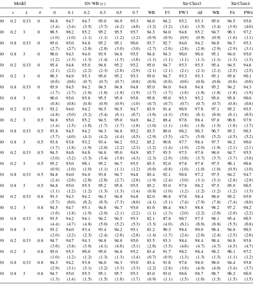
Table 4. Percentages of coverage of the 95% confidence intervals (mean lengths of the interval in the parentheses) of the linear trend model (7) with (b1,b2)=(0, 5), (A1)–MA(1), single volatility shifts. The number of replications is 2000, and 1000 pseudoseries with iidN(0, 1) are used
for the wild bootstrap
Model SN-WB (ǫ) Xu-Class3 Xu-Class4
n τ δ θ 0 0.1 0.2 0.3 0.5 0.7 WB F3 PW3 iid WB F4 PW4
100 0.2 0.33 0 94.8 94.7 94.7 95.0 94.9 95.3 94.0 94.2 95.2 95.3 95.0 94.5 95.0 (3.4) (3.4) (3.5) (3.7) (4.2) (4.6) (3.2) (3.2) (3.4) (3.5) (3.4) (3.9) (4.0) 100 0.2 3 0 96.5 96.2 95.2 95.2 95.5 95.7 94.3 94.0 94.8 95.2 94.7 96.1 97.2
(1.0) (1.0) (1.1) (1.1) (1.2) (1.2) (0.9) (0.9) (0.9) (0.9) (0.9) (1.0) (1.1) 100 0.8 0.33 0 95.0 95.0 94.8 95.2 95.1 96.0 93.7 92.7 94.0 94.2 94.6 94.7 95.3
(2.7) (2.7) (2.8) (2.8) (3.0) (3.0) (2.7) (2.6) (2.8) (2.8) (2.9) (2.9) (3.1) 100 0.8 3 0 96.0 94.3 94.0 93.9 94.8 95.5 94.8 94.3 96.0 96.0 95.1 94.0 95.0
(1.2) (1.3) (1.3) (1.4) (1.5) (1.6) (1.1) (1.1) (1.1) (1.1) (1.1) (1.3) (1.3) 250 0.2 0.33 0 95.4 94.8 95.0 94.8 95.2 95.2 95.0 94.7 95.3 95.5 95.4 94.5 94.8
(2.1) (2.2) (2.2) (2.3) (2.6) (2.9) (2.1) (2.1) (2.1) (2.1) (2.1) (2.5) (2.5) 250 0.2 3 0 96.3 94.9 95.3 95.0 95.2 95.3 95.0 94.7 95.3 95.3 95.1 95.8 96.1
(0.6) (0.6) (0.7) (0.7) (0.7) (0.8) (0.6) (0.6) (0.6) (0.6) (0.6) (0.6) (0.6) 250 0.8 0.33 0 95.9 94.5 94.2 94.5 94.8 94.8 95.0 94.0 94.8 94.8 95.2 94.2 94.3
(1.7) (1.7) (1.8) (1.8) (1.8) (1.9) (1.7) (1.7) (1.8) (1.8) (1.8) (1.8) (1.9) 250 0.8 3 0 96.0 95.0 95.8 95.5 95.9 95.6 95.6 95.0 95.3 95.2 95.0 95.8 96.0
(0.8) (0.8) (0.8) (0.9) (0.9) (1.0) (0.7) (0.7) (0.7) (0.7) (0.7) (0.8) (0.8) 100 0.2 0.33 0.5 93.2 94.0 94.2 94.5 94.5 94.7 83.9 91.4 96.9 97.6 97.1 95.2 95.5
(4.8) (5.0) (5.2) (5.4) (6.1) (6.7) (3.6) (4.3) (5.8) (6.1) (6.0) (6.1) (6.5) 100 0.2 3 0.5 94.8 95.0 95.2 94.5 95.0 94.9 84.2 89.4 97.6 98.4 97.8 96.6 97.9
(1.4) (1.5) (1.6) (1.7) (1.7) (1.8) (1.0) (1.1) (1.6) (1.6) (1.5) (1.6) (1.7) 100 0.8 0.33 0.5 93.8 94.5 94.2 94.3 94.8 95.2 83.5 89.0 96.2 96.3 96.7 95.2 96.3
(3.7) (4.0) (4.1) (4.2) (4.4) (4.5) (2.9) (3.5) (4.7) (5.0) (5.2) (4.5) (5.2) 100 0.8 3 0.5 93.8 93.8 93.2 93.4 94.2 95.2 85.2 90.6 97.7 98.4 97.7 94.2 96.0
(1.7) (1.8) (1.9) (2.0) (2.2) (2.3) (1.2) (1.4) (1.9) (2.0) (1.9) (2.1) (2.1) 250 0.2 0.33 0.5 94.5 94.6 94.6 94.8 95.0 94.9 85.7 93.5 97.5 97.8 98.0 94.7 95.5
(3.0) (3.2) (3.3) (3.4) (3.8) (4.3) (2.3) (2.9) (3.6) (3.7) (3.7) (3.7) (3.8) 250 0.2 3 0.5 95.2 95.0 96.1 95.2 94.7 95.5 85.5 92.0 97.8 97.8 97.5 96.1 96.8
(0.9) (1.0) (1.0) (1.1) (1.1) (1.2) (0.6) (0.8) (1.0) (1.0) (1.0) (0.9) (1.0) 250 0.8 0.33 0.5 94.8 94.0 94.0 93.8 94.7 94.8 85.4 92.1 96.8 97.2 97.5 94.2 94.7
(2.4) (2.6) (2.6) (2.6) (2.7) (2.8) (1.9) (2.4) (3.0) (3.1) (3.1) (2.8) (2.9) 250 0.8 3 0.5 94.8 95.0 95.5 95.2 95.8 95.5 85.2 93.0 97.8 98.2 97.5 95.9 96.5
(1.1) (1.2) (1.2) (1.3) (1.3) (1.4) (0.8) (1.0) (1.2) (1.2) (1.2) (1.2) (1.3) 100 0.2 0.33 0.8 93.3 94.3 94.2 94.3 94.8 94.8 82.0 90.8 97.6 98.4 98.0 95.2 95.9
(5.7) (6.0) (6.2) (6.5) (7.3) (8.0) (4.1) (5.1) (7.4) (7.9) (7.8) (7.4) (8.0) 100 0.2 3 0.8 94.5 94.7 95.1 94.6 94.7 95.0 81.6 88.4 98.3 98.8 98.2 97.2 98.2
(1.6) (1.8) (1.9) (2.0) (2.1) (2.2) (1.1) (1.3) (2.0) (2.2) (2.0) (2.0) (2.2) 100 0.8 0.33 0.8 93.5 94.2 94.1 94.2 94.5 95.3 82.1 87.8 96.7 97.5 98.1 95.4 96.5
(4.4) (4.7) (4.8) (5.0) (5.2) (5.3) (3.3) (4.0) (6.1) (6.6) (6.8) (5.5) (6.8) 100 0.8 3 0.8 93.2 94.0 93.4 93.4 94.2 95.1 83.2 90.3 98.4 99.0 98.4 94.8 96.5
(2.0) (2.2) (2.3) (2.4) (2.6) (2.8) (1.4) (1.7) (2.4) (2.6) (2.4) (2.5) (2.6) 250 0.2 0.33 0.8 94.7 94.7 94.3 94.8 94.8 95.0 83.5 93.3 98.4 98.4 98.4 94.8 95.8
(3.6) (3.8) (3.9) (4.1) (4.6) (5.1) (2.6) (3.5) (4.6) (4.7) (4.7) (4.5) (4.7) 250 0.2 3 0.8 95.0 95.3 96.0 95.0 94.8 95.2 83.4 91.7 98.2 98.4 98.2 96.1 97.2
(1.0) (1.2) (1.2) (1.3) (1.3) (1.4) (0.7) (0.9) (1.3) (1.3) (1.3) (1.1) (1.2) 250 0.8 0.33 0.8 94.3 94.2 93.8 94.0 94.3 95.0 83.4 91.6 97.8 98.0 98.0 94.4 95.8
(2.9) (3.1) (3.1) (3.2) (3.3) (3.3) (2.2) (2.8) (3.8) (4.0) (4.0) (3.4) (3.7) 250 0.8 3 0.8 94.7 95.0 95.5 95.1 95.7 95.3 83.0 93.0 98.6 98.7 98.7 96.2 96.9
(1.3) (1.4) (1.5) (1.5) (1.6) (1.7) (0.9) (1.1) (1.5) (1.6) (1.5) (1.5) (1.5)
have more accurate coverage rates regardless of the choice of the trimming parameterǫ. Not surprisingly, prewhitening is very effective in bringing the coverage level closer to the nominal level. Xu’s Class 4 test seems to provide the best coverage rates, for both prewhitened and nonprewhitened versions.
However, Xu’s methods and his prewhitening are based on the assumption that the errors are from an AR model with a known lag. When the errors are not from an AR model, then the performance may deteriorate. As can be seen from Table 4, where the errors are generated from an MA model,
Table 5. Percentages of coverage of the 95% confidence intervals ofb2(mean lengths of the interval in the parentheses) of the linear trend
model with a break in intercept (8) with (b1,b2,b3)=(0, 2, 5), (A1)–AR(1), single volatility shifts. The number of replications is 2000, and
1000 pseudoseries with iidN(0, 1) are used for the wild bootstrap
Model SN-WB (ǫ)
n τ δ ρ 0.35 0.4 0.5 0.6 0.7 WB HAC
100 0.2 0.33 0 94.5 94.5 94.3 94.8 94.8 94.0 93.0
(5.5) (5.5) (5.6) (5.7) (5.9) (3.9) (3.8)
100 0.2 3 0 94.6 94.7 95.0 95.0 95.4 94.4 94.5
(1.1) (1.1) (1.1) (1.0) (1.0) (0.6) (0.6)
100 0.8 0.33 0 95.0 95.0 95.1 95.3 95.5 94.5 93.6
(2.4) (2.4) (2.4) (2.5) (2.5) (1.9) (1.9)
100 0.8 3 0 94.2 94.2 94.3 94.7 94.7 93.3 93.2
(2.0) (2.0) (2.0) (2.0) (2.2) (1.3) (1.3)
250 0.2 0.33 0 95.6 95.6 95.5 95.5 95.1 94.2 94.2
(3.6) (3.6) (3.6) (3.6) (3.7) (2.5) (2.5)
250 0.2 3 0 95.0 95.0 95.0 94.8 94.8 94.5 94.6
(0.7) (0.7) (0.7) (0.6) (0.6) (0.4) (0.4)
250 0.8 0.33 0 95.8 95.8 95.8 95.9 95.8 94.3 94.0
(1.5) (1.5) (1.5) (1.5) (1.5) (1.2) (1.2)
250 0.8 3 0 95.0 95.0 94.8 95.1 95.6 94.2 94.2
(1.3) (1.3) (1.3) (1.3) (1.4) (0.8) (0.8)
100 0.2 0.33 0.5 93.7 93.8 93.8 93.3 93.0 73.1 84.6
(10.1) (10.1) (10.1) (10.3) (10.6) (4.3) (5.7)
100 0.2 3 0.5 93.9 93.8 93.8 94.0 93.5 71.9 87.4
(2.0) (2.0) (2.0) (2.0) (1.9) (0.7) (1.0)
100 0.8 0.33 0.5 93.7 93.7 93.7 93.5 93.5 71.9 84.9
(4.5) (4.5) (4.5) (4.5) (4.5) (2.1) (2.8)
100 0.8 3 0.5 93.2 93.2 93.2 93.1 93.0 72.1 84.3
(3.6) (3.6) (3.6) (3.7) (4.0) (1.4) (1.9)
250 0.2 0.33 0.5 95.1 95.2 95.2 94.9 94.7 73.4 88.5
(6.8) (6.8) (6.9) (7.0) (7.2) (2.8) (4.2)
250 0.2 3 0.5 94.0 94.0 93.8 94.0 94.3 72.0 89.5
(1.3) (1.3) (1.3) (1.3) (1.2) (0.5) (0.7)
250 0.8 0.33 0.5 95.4 95.4 95.2 95.0 95.0 74.2 88.8
(2.9) (2.9) (2.9) (2.9) (2.9) (1.4) (2.1)
250 0.8 3 0.5 94.5 94.5 94.5 94.7 95.2 72.5 88.5
(2.4) (2.4) (2.4) (2.5) (2.7) (0.9) (1.4)
100 0.2 0.33 0.8 91.0 91.0 91.0 90.8 90.1 47.9 72.5
(20.2) (20.2) (20.3) (20.8) (21.3) (5.6) (9.8)
100 0.2 3 0.8 90.8 90.9 91.0 91.0 89.8 42.9 71.4
(4.4) (4.4) (4.3) (4.2) (4.1) (1.0) (1.8)
100 0.8 0.33 0.8 93.2 93.2 93.0 92.6 92.0 46.0 74.9
(9.3) (9.3) (9.3) (9.3) (9.3) (2.8) (4.9)
100 0.8 3 0.8 92.5 92.4 92.2 92.4 92.5 47.4 72.9
(7.3) (7.3) (7.3) (7.6) (8.0) (1.9) (3.3)
250 0.2 0.33 0.8 93.7 93.7 93.9 94.0 94.1 48.9 81.9
(15.4) (15.4) (15.5) (15.8) (16.2) (3.9) (8.4)
250 0.2 3 0.8 91.8 92.0 92.0 92.0 92.4 45.2 82.1
(3.1) (3.1) (3.0) (3.0) (2.9) (0.7) (1.5)
250 0.8 0.33 0.8 93.5 93.5 93.4 93.8 93.3 48.6 82.8
(6.7) (6.7) (6.7) (6.7) (6.7) (1.9) (4.2)
250 0.8 3 0.8 93.5 93.5 93.4 93.6 94.2 48.0 81.2
(5.5) (5.5) (5.5) (5.7) (6.1) (1.3) (2.8)
in some cases Xu’s tests, except for his test 3, tend to provide overcoverage, especially whenδ =3. On the other hand, our SN-WB method tends to provide more stable results. Further-more, in our unreported simulations, when the order of the VAR model is misspecified, Xu’s methods can be sensitive to the form of misspecification. Thus, when the true model of the error pro-cess is not VAR or true order of the VAR model is not known, Xu’s methods may not be advantageous.
In this linear trend assessment setting, we need to useǫ >0 so that our method is theoretically valid. As can be seen inTable 3, if the dependence is weak or moderate (ρ=0 or 0.5), the choice ofǫdoes not affect the coverage accuracy much, andǫ=0.1 or above seems appropriate. However, the effect ofǫ is more apparent when the dependence is stronger, that is, whenρ =0.8. It seems thatǫ∈ {0.2,0.3,0.4}are all reasonable choices here, considering the amount of improvement in coverage percentage. Notice that even when our choice ofǫis not optimal, the SN-WB method delivers more accurate coverage than the HAC method. In terms of the interval length, there is a mild monotonic relationship betweenǫand interval length. The largerǫis, the longer the interval tends to become. As a rule of thumb in practice, we can useǫ∈[0.2,0.4] if the temporal dependence in the data is likely to be strong, otherwise, we can also useǫ=0.1, which was also recommended by Zhou and Shao (2013) under a different setting.
4.3 Linear Trend Models With a Break in Intercept
This section concerns the linear trend models with a break in its mean level at a known point,
Xt,n=b1+b21(t /n > sb)+b3(t /n)+ut,n, t =1, . . . , n, (8)
wheresb ∈(0,1) indicates the relative location for the intercept break, which is assumed to be known. Without loss of generality, letsb =0.3,b1=0, b2=2,andb3=5, which was modified
from the model we fit in the data illustration in Section5. Our interest is on constructing confidence intervals for the break pa-rameterb2. For the error process{ut,n}, we use the AR(1) model, as introduced in the second simulation of Section4.1. Because of the general form of the trend function, neither Xu’s nor Zhao’s methods work in this setting. Here, we compare the HAC-type method defined in (4) with our SN-WB(ǫ) method, and the wild bootstrap alone. For the HAC-type method, the bandwidth pa-rameter is chosen following Andrews’ (1991) suggestion for the AR(1) model, so in a sense, this HAC-type method takes some advantage of the knowledge of the true model.
Table 5presents the empirical coverage rates for 95% confi-dence intervals ofb2. The mean interval lengths are in
parenthe-ses. When there is no temporal dependence, that is,ρ=0, all methods work well. When there is moderate (ρ=0.5) or strong (ρ=0.8) dependence, the wild bootstrap is no longer consis-tent. In this case, the HAC method with Andrews’ bandwidth parameter choice also shows some departures from the nomi-nal level, converging to its limit much slower than our method. In this setting, our SN-WB method provides the most accurate coverage rates. Even the worst coverage of our SN-WB method for a range ofǫ’s under examination seems to be more accurate than the HAC method in all simulation settings. Notice that for this kind of linear trend model with a break in the intercept, the trimming parameterǫin our method should be chosen so that
ǫ > sb. See Remark 3.2 for more details. In this simulation, sincesb=0.3, we chooseǫto be 0.35, 0.4, 0.5, 0.6, and 0.7. The results does not seem to be sensitive to the choice of this trimming parameter.
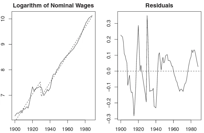
5. DATA ANALYSIS
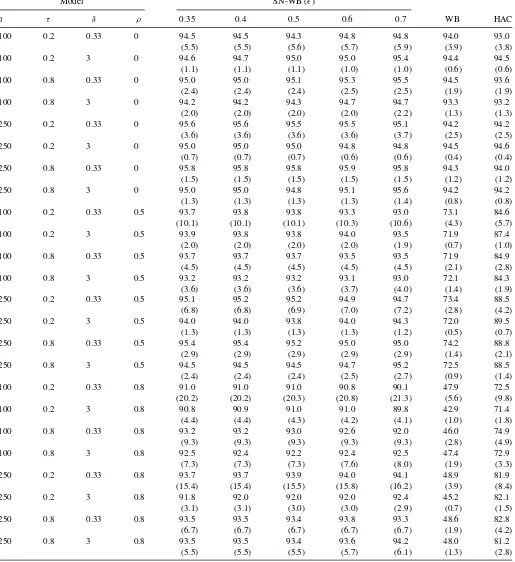
In this section, we illustrate our method using the logarithm of the U.S. nominal wage data, which was originally from Nelson and Plosser (1982) for the period 1900–1970 and has been in-tensively analyzed in econometrics literature, including Perron (1989). The latter author argued that this series has a fairly stable
Logarithm of Nominal Wages
1900 1920 1940 1960 1980
789
1
0
Residuals
1900 1920 1940 1960 1980
−0.3
−0.2
−0.1
0.0
0.1
0.2
0.3
Figure 1. The nominal wage series fitted with a break at 1929 (the Great Crash) and the corresponding residuals.
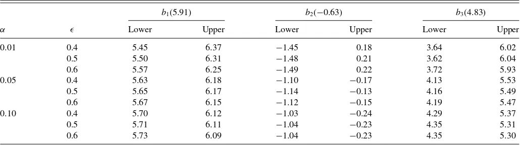
Table 6. The 100(1−α)% confidence intervals for the parameters in the model (9) for the nominal wage series. The estimated coefficients are shown in the parenthesis
b1(5.91) b2(−0.63) b3(4.83)
α ǫ Lower Upper Lower Upper Lower Upper
0.01 0.4 5.45 6.37 −1.45 0.18 3.64 6.02
0.5 5.50 6.31 −1.48 0.21 3.62 6.04
0.6 5.57 6.25 −1.49 0.22 3.72 5.93
0.05 0.4 5.63 6.18 −1.10 −0.17 4.13 5.53
0.5 5.65 6.17 −1.14 −0.13 4.16 5.49
0.6 5.67 6.15 −1.12 −0.15 4.19 5.47
0.10 0.4 5.70 6.12 −1.03 −0.24 4.29 5.37
0.5 5.71 6.11 −1.04 −0.23 4.35 5.31
0.6 5.73 6.09 −1.04 −0.23 4.35 5.30
linear trend with a sudden decrease in level between 1929 and 1930 (the Great Crash). In this section, we examine his assertion for an extended dataset for the period 1900–1988, provided by Koop and Steel (1994). The left panel ofFigure 1presents the data fitted with the linear trend model with one break in the intercept
Xt,n=b1+b21(t >30)+b3(t /n)+ut,n, t=1, . . . , n=89. (9)
Here the second regressor 1(t >30) represents the break at year 1929. From the residual plot on the right panel ofFigure 1, the error appears to exhibit some degree of heteroscedastic-ity. Our inference method, which is robust to this kind of het-eroscedasticity and weak temporal dependence, is expected to be more appropriate than other existing methods, the validity of which hinges on the stationarity of the errors.Table 6reports the 100(1−α)% confidence intervals withα=0.01,0.05,0.1, for the three coefficients using our method. For the wild bootstrap, we used 1000 pseudoseries{Wt}nt=1drawn from iidN(0,1). For
the choice of the trimming parameterǫ, we useǫ=0.4,0.5,0.6. Note that since there is a break in the regressor at 30/89=0.34,
ǫcannot be less than 0.34, see Remark 3.2. As can be seen in Ta-ble 6, the resulting confidence intervals are not very sensitive to the choice of the trimming parameterǫ. In fact, the confidence intervals unanimously suggest that the linear trend is signifi-cantly positive, that is, the nominal wage is linearly increasing at significance level 1% with a 99% confidence interval of about [3.6,6], and the decrease at the Great Crash is significant at 5% level but not at 1% level.
6. CONCLUSION
In this article, we study the estimation and inference of non-stationary time series regression models by extending the SN method (Lobato 2001; Shao 2010) to the regression setting with fixed parametric regressors and weakly dependent non-stationary errors with unconditional heteroscedasticity. Due to the heteroscedasticity and nonconstant regressor, the limiting distribution of the SN quantity is no longer pivotal and con-tains a number of nuisance parameters. To approximate the limiting distribution, we apply the wild bootstrap (Wu 1986) and rigorously justify its consistency. Simulation comparison
demonstrates the advantage of our method in comparison with HAC-based alternatives. The necessity of self-normalization is also demonstrated in theory and finite samples.
The two kinds of heteroscedastic time series models we con-sider in this article are natural generalizations of the classical linear process and the stationary causal process to capture un-conditional heteroscedasticity often seen on the data. However, it is restricted only to the short-range dependence as seen from our condition (A1) (ii) and (A2) (iii). When there is long-range dependence, it is not clear if the SN method is still applicable. This can be an interesting topic for future research. Further-more, the OLS is a convenient but not an efficient estimator of the regression parameter when the errors exhibit autocorrelation and heteroscedasticity. How to come up with a more efficient estimator and perform the SN-based inference is worthy of a careful investigation. Finally, our method assumes a parametric form for the mean function so it is easy to interpret and the prediction is straightforward. However, a potential drawback is that the result may be biased if the parametric trend function is misspecified. We can avoid this misspecification problem by preapplying Zhang and Wu’s (2011) test to see if a parametric form fits the data well. The inferential procedure developed here can be readily used provided that a suitable parametric form is specified.
SUPPLEMENTARY MATERIALS
Technical Appendix: Proofs of Theorems 3.1 and 3.2. (pdf file)
ACKNOWLEDGMENTS
The research is supported in part by NSF grants DMS08-04937 and DMS11-04545. The authors are grateful to the refer-ees for constructive comments that led to a substantial improve-ment of the article.
[Received September 2013. Revised July 2014.]
REFERENCES
Andrews, D. W. K. (1991), “Heteroskedasticity and Autocorrelation Consistent Covariance Matrix Estimation,”Econometrica, 59, 817–858. [446,451,455]
Billingsley, P. (1968),Convergence of Probability Measures, New York: Wiley. [445]
Bunzel, H., and Vogelsang, T. (2005), “Powerful Trend Function Tests That are Robust to Strong Serial Correlation, With an Application to the Prebisch-Singer Hypothesis,”Journal of Business and Economic Statistics, 23, 381– 394. [444]
Busetti, F., and Taylor, R. (2003), “Variance Shifts, Structural Breaks, and Stationarity Tests,”Journal of Business and Economic Statistics, 21, 510– 531. [444]
Canjels, E., and Watson, M. W. (1997), “Estimating Deterministic Trends in the Presence of Serially Correlated Errors,”The Review of Economics and Statistics, 79, 184–200. [444]
Cavaliere, G. (2005), “Unit Root Tests Under Time-Varying Variances,” Econo-metric Reviews, 23, 259–292. [446]
Cavaliere, G., and Taylor, A. M. R. (2007), “Testing for Unit Roots in Time Series Models With Non-Stationary Volatility,”Journal of Econometrics, 140, 919–947. [445,446,450]
——— (2008a), “Time-Transformed Unit Root Tests for Models With Non-Stationary Volatility,” Journal of Time Series Analysis, 29, 300– 330. [445,446,450]
——— (2008b), “Bootstrap Unit Root Tests for Time Series With Nonstationary Volatility,”Econometric Theory, 24, 43–71. [445,446,450]
Dahlhaus, R. (1997), “Fitting Time Series Models to Nonstationary Processes,” The Annals of Statistics, 25, 1–37. [445]
Fitzenberger, B. (1998), “The Moving Blocks Bootstrap and Robust Inference for Linear Least Squares and Quantile Regressions,”Journal of Economet-rics, 82, 235–287. [446]
Hamilton, J. D. (1994),Time Series Analysis, Princeton: Princeton University Press. [444]
Harvey, D. I., Leybourne, S. J., and Taylor, A. M. R. (2007), “A Simple, Robust and Powerful Test of the Trend Hypothesis,”Journal of Econometrics, 141, 1302–1330. [444]
Kiefer, N. M., and Vogelsang, T. (2005), “A New Asymptotic Theory for Heteroskedasticity-Autocorrelation Robust Tests,”Econometric Theory, 21, 1130–1164. [447]
Kiefer, N. M., Vogelsang, T., and Bunzel, H. (2000), “Simple Robust Testing of Regression Hypotheses,”Econometrica, 68, 695–714. [447,448,449] Kim, C.-J., and Nelson, C. R. (1999), “Has the U.S. Economy Become
More Stable? A Bayesian Approach Based on a Markov-Switching Model of the Business Cycle,” The Review of Economics and Statistics, 81, 608–616. [444]
Koop, G., and Steel, M. (1994), “A Decision-Theoretic Analysis of the Unit-Root Hypothesis Using Mixtures of Elliptical Models,”Journal of Business and Economic Statistics, 12, 95–107. [456]
Lahiri, S. N. (2003),Resampling Methods for Dependent Data, New York: Springer. [446]
Lobato, I. N. (2001), “Testing That a Dependent Process is Uncorre-lated,” Journal of the American Statistical Association, 96, 1066– 1076. [445,447,448,456]
Mammen, E. (1993), “Bootstrap and Wild Bootstrap for High Dimensional Linear Models,”The Annals of Statistics, 21, 255–285. [448,450] McConnell, M. M., and Perez-Quiros, G. (2000), “Output Fluctuations in the
United States: What has Changed Since the Early 1980’s?”American Eco-nomic Review, 90, 1464–1476. [444]
Nelson, C. R., and Plosser, C. I. (1982), “Trends and Random Walks in Macroe-conomic Time Series : Some Evidence and Implications,”Journal of Mon-etary Economics, 10, 139–162. [455]
Newey, W., and West, K. D. (1987), “A Simple, Positive Semi-Definite, Het-eroskedasticity and Autocorrelation Consistent Covariance Matrix,” Econo-metrica, 55, 703–708. [446]
Paparoditis, E., and Politis, D. N. (2002), “Local Block Bootstrap,”Comptes Rendus Mathematique, 335, 959–962. [446]
Perron, P. (1989), “The Great Crash, the Oil Price Shock, and the Unit Root Hypothesis,”Econometrica, 57, 1361–1401. [444,455]
Politis, D. N., Romano, J. P., and Wolf, M. (1999),Subsampling, New York: Springer. [446]
Priestley, M. B. (1965), “Evolutionary Spectra and Non-Stationary Processes,” Journal of the Royal Statistical Society,Series B, 27, 204–237. [445] Rao, S. S. (2004), “On Multiple Regression Models With Nonstationary
Corre-lated Errors,”Biometrika, 91, 645–659. [444]
Rho, Y., and Shao, X. (2013), “Improving the Bandwidth-Free Inference Meth-ods by Prewhitening,”Journal of Statistical Planning and Inference, 143, 1912–1922. [447,448,449]
Romano, J. P., and Wolf, M. (2006), “Improved Nonparametric Confidence Intervals in Time Series Regressions,”Journal of Nonparametric Statistics, 18, 199–214. [446]
Sensier, M., and van Dijk, D. (2004), “Testing for Volatility Changes in U.S. Macroeconomic Time Series,”The Review of Economics and Statistics, 86, 833–839. [444]
Shao, X. (2010), “A Self-Normalized Approach to Confidence Interval Con-struction in Time Series,”Journal of the Royal Statistical Society,Series B, 72, 343–366. [445,447,456]
Sherman, M. (1997), “Subseries Methods in Regression,”Journal of the Amer-ican Statistical Association, 92, 1041–1048. [444,446]
Stock, J., and Watson, M. (1999), “A Comparison of Linear and Nonlin-ear Univariate Models for Forecasting Macroeconomic Time Series,” in Cointegration, Causality and Forecasting: A Festschrift for Clive W.J. Granger, eds. R. Engle and H. White, Oxford: Oxford University Press, pp. 1–44. [444]
Vogelsang, T. (1998), “Trend Function Hypothesis Testing in the Presence of Serial Correlation,”Econometrica, 66, 123–148. [444]
Wu, C. F. J. (1986), “Jackknife, Bootstrap and Other Resampling Methods in Regression Analysis” (with discussion),The Annals of Statistics, 14, 1261– 1350. [445,448,456]
Wu, W. B. (2005), “Nonlinear System Theory: Another Look at Dependence,” Proceedings of the National Academy of Sciences of the United States of America, 102, 14150–14154. [444,446]
Xu, K.-L. (2008), “Bootstrapping Autoregression Under Non-Stationary Volatil-ity,”Econometrics Journal, 11, 1–26. [444]
——— (2012), “Robustifying Multivariate Trend Tests to Nonstationary Volatil-ity,”Journal of Econometrics, 169, 147–154. [444,448,449,451]
Xu, K.-L., and Phillips, P. C. (2008), “Adaptive Estimation of Autoregressive Models With Time-Varying Variances,”Journal of Econometrics, 142, 265– 280. [444,446]
Zhang, T., and Wu, W. B. (2011), “Testing Parametric Assumptions of Trends of a Nonstationary Time Series,”Biometrika, 98, 599–614. [444] Zhao, Z. (2011), “A Self-Normalized Confidence Interval for the Mean of a
Class of Nonstationary Processes,”Biometrika, 98, 81–90. [444,446,449] Zhao, Z., and Li, X. (2013), “Inference for Modulated Stationary Processes,”
Bernoulli, 19, 205–227. [444,445,446,448]
Zhou, Z., and Shao, X. (2013), “Inference for Linear Models With De-pendent Errors,”Journal of the Royal Statistical Society, Series B, 75, 323–343. [444,445,447,448,455]
Zhou, Z., and Wu, W. B. (2009), “Local Linear Quantile Estimation for Non-stationary Time Series,”The Annals of Statistics, 37, 2696–2729. [444]