Full Terms & Conditions of access and use can be found at
http://www.tandfonline.com/action/journalInformation?journalCode=ubes20
Download by: [Universitas Maritim Raja Ali Haji] Date: 11 January 2016, At: 19:16
Journal of Business & Economic Statistics
ISSN: 0735-0015 (Print) 1537-2707 (Online) Journal homepage: http://www.tandfonline.com/loi/ubes20
Testing Instantaneous Causality in Presence
of Nonconstant Unconditional Covariance
Quentin Giai Gianetto & Hamdi Raïssi
To cite this article: Quentin Giai Gianetto & Hamdi Raïssi (2015) Testing Instantaneous Causality in Presence of Nonconstant Unconditional Covariance, Journal of Business & Economic Statistics, 33:1, 46-53, DOI: 10.1080/07350015.2014.920614
To link to this article: http://dx.doi.org/10.1080/07350015.2014.920614
View supplementary material
Accepted author version posted online: 21 May 2014.
Submit your article to this journal
Article views: 138
View related articles
Testing Instantaneous Causality in Presence
of Nonconstant Unconditional Covariance
Quentin G
IAIG
IANETTOand Hamdi R
A¨
ISSIIRMAR-INSA, F-35708 Rennes, France ([email protected])
This article investigates the problem of testing instantaneous causality between vector autoregressive (VAR) variables with time-varying unconditional covariance. It is underlined that the standard test does not control the Type I errors, while the tests with White and heteroscedastic autocorrelation consistent (HAC) corrections can suffer from a severe loss of power when the covariance is not constant. Consequently, we propose a modified test based on a bootstrap procedure. We illustrate the relevance of the modified test through a simulation study. The tests considered in this article are also compared by investigating the instantaneous causality relations between U.S. macroeconomic variables.
KEY WORDS: Unconditionally heteroscedastic errors; VAR model; Wild bootstrap.
1. INTRODUCTION
The concept of Granger causality (Granger1969) has evolved as a standard tool to analyze cause-and-effect relationships be-tween variables. Seminal papers relying on this concept are Sims (1972), Ashenfelter and Card (1982), Hamilton (1983), Lee (1992), and Hiemstra and Jones (1994) among others. In particular, it is said that there exists aninstantaneouscausality relation betweenX1t andX2t if the prediction ofX2t given the
past values ofXt=(X1′t, X′2t)′is improved by adding the
avail-able current information of the variavail-ables inX1t(see L¨utkepohl
2005, p. 42). WhenXt is assumed to follow a VAR process, a
standard Wald test for zero restrictions on the errors covariance matrix is usually used for testing the instantaneous causality. Such a test, available in most specialized software, is based on the assumption of iid Gaussian errors (see L¨utkepohl and Kr¨atzig 2004). In nonstandard stationary cases, White (White1980) or HAC corrections are considered (see Den Haan and Levin1997 for the HAC estimation). Such situations arise when the error process is non-Gaussian or dependent. For instance nonlinear models are often adjusted to residuals (see, e.g., Bauwens, Lau-rent, and Rombouts2006; Andrews, Davis, and Jay Breidt2006; Amendola and Francq2009for nonlinear processes).
The Wald test and its corrections assume a constant uncon-ditional covariance structure that has been challenged through many statistical studies applied to real data. For instance, Sensier and Van Dijk (2004) found that most of the 214 U.S. macroe-conomic variables they investigated exhibit a break in their un-conditional variance. Ramey and Vine (2006) highlighted a de-clining variance of the U.S. automobile production and sales. McConnell and Perez-Quiros (2000) documented a break in variance in the U.S. GDP growth and pointed out that neglect-ing nonconstant variance can be misleadneglect-ing for the data anal-ysis. In the literature numerous tools for time series analysis in presence of nonconstant variance have been proposed. For instance Tsay (1988), Horv`ath, Kokoszka, and Zhang (2006), or Sans´o, Arag´o, and Carrion (2004) proposed tests for detect-ing unconditional variance changes in several situations. Li and Zhao (2013) developed a test procedure for detecting changes in the autocovariance structure based on the theoretical frame-work of Wu (2007). Robinson (1987) or Xu and Phillips (2008)
among others investigated univariate linear models allowing for a nonconstant variance. St˘aric˘a (2004) considered a deter-ministic nonconstant unconditional variance of stock returns, and noticed that such an approach can perform as well as the stationary GARCH(1,1) model for forecasting purposes. Kim and Park (2010) studied cointegrated systems with nonconstant covariance. Bai (2000), Qu and Perron (2007), and Patilea and Ra¨ıssi (2012) among others investigated the estimation of multi-variate models with time-varying covariance. Aue et al. (2009) proposed a test procedure for detecting covariance breaks in multivariate time series.
In this article we focus on the test of zero restrictions on time-varying covariance structure of the VAR innovations. Var-ious forms of nonconstant unconditional variance specifications have been considered in the literature. For instance Francq and Gautier (2004) studied linear models allowing for unconditional changes in the variance driven by a Markov chain. Engle and Rangel (2008) and Hafner and Linton (2010) proposed deter-ministic changes of the unconditional variance combined with a GARCH structure. Kokoszka and Leipus (2000) and Dahlhaus and Rao (2006) studied ARCH processes with time-varying pa-rameters. Hansen (1995) assumed that the volatility is driven by a near integrated process. In the above contributions, the nonconstant unconditional variance is subject to stochastic ef-fects. Reference can be also made to Azrak and Melard (2006) who investigated the estimation of ARMA models with possi-ble nonconstant deterministic unconditional variance. Zhao and Li (2013) considered a deterministic general form of noncon-stant variance which allows for nonlocally stationary processes. In this article the rescaling device of Dahlhaus (1997) is used for the deterministic covariance structure (see Assumption A1). This kind of time-varying covariance specification is widely used in the literature and encompasses the piecewise constant case (see Hamori and Tokihisa1997; Pesaran and Timmermann 2004; or Xu and Phillips2008and references therein). In this
© 2015American Statistical Association
Journal of Business & Economic Statistics January 2015, Vol. 33, No. 1 DOI:10.1080/07350015.2014.920614
46
Giai Gianetto and Ra¨ıssi: Testing Instantaneous Causality in Presence of Nonconstant Unconditional Covariance 47
framework, it is highlighted that the standard Wald test for in-stantaneous causality does not provide suitable critical values. To remove such undesirable effects of heteroscedasticity, it is common to consider a White correction or apply a wild bootstrap procedure on the standard test statistic. However, it emerges that the tests with White or HAC corrections can suffer from a se-vere loss of power. It also appears that applying a wild bootstrap procedure directly to the standard statistic does not solve the problem. Noticing that the previous approaches fail to handle data with nonconstant covariance, we propose a new test for in-vestigating instantaneous causality based on cumulative sums. We find that the asymptotic distribution of the corresponding statistic is nonstandard involving the unknown nonconstant co-variance structure in a functional form. Therefore, we develop a wild bootstrap procedure to propose accurate critical values for our task (see, e.g., Wu1986; Gonc¸alvez and Kilian2004; Horowitz et al.2006; Inoue and Kilian2002for the wild boot-strap method). We establish through theoretical and empirical results that the modified test is preferable to the tests based on the spurious assumption of stationary time series.
The plan of the article is as follows. In Section2the VAR model with nonconstant covariance is introduced. The proper-ties of the tests based on the assumption of constant uncondi-tional covariance are given. It emerges from this part that this kind of tests should be avoided in our nonstandard framework. As a consequence a test based on the wild bootstrap procedure taking into consideration nonconstant covariance is proposed in Section3. The finite sample properties of the tests are in-vestigated in Section4by Monte Carlo experiments. Outcomes obtained from U.S. macroeconomic datasets illustrate our find-ings. In Section5, we draw up a conclusion on our results.
The following general notations will be used. The conver-gence in distribution will be denoted by⇒, while→denotes the convergence in probability. The usual Kronecker product between matrices is denoted by⊗. The usual operator which stacks the columns of a given matrix into a vector is signified by vec(.). For a random variablexwe definexr:=(Ex r)1/r
where.is the Euclidean norm. A d×d identity matrix is denoted byId.
2. VAR MODEL WITH NONCONSTANT COVARIANCE
Let Xt =(X′1t, X2′t)′∈R
sive order p is supposed to be known to state the asymptotic results and to assess their finite sample reliability, eliminating the effects of a misspecification ofp(Sections2,3, and4.1). Of course, in practice, the lag length is unknown. For instance, we select it using a goodness-of-fit test taking into account the time-varying covariance in the real data study (Section4.2). The case where the lag length is adjusted before testing for instantaneous causality is investigated in the online supplementary material
through Monte Carlo experiments. The nonconstant covariance induced byHtis specified in A1:
Assumption A1. (i) The d×d matrices Ht are lower
tri-angular nonsingular matrices with positive diagonal elements and satisfyHt=G(t /T), where the components of the matrix
G(r) := {gkl(r)}are measurable deterministic functions on the
interval (0,1], such that supr∈(0,1]|gkl(r)|<∞, and each gkl
satisfies a Lipschitz condition piecewise on a finite number of subintervals partitioning (0,1]. The matrices(r)=G(r)G(r)′ are assumed positive definite for allrin (0,1].
(ii) (ǫt) is α-mixing, such that E(ǫt|Ft−1)=0, E(ǫtǫt′|
Ft−1)=Id, whereFt is theσ-field generated by{ǫk:k≤t},
and supt ǫt 4µ<∞for someµ >1.
Since the rescaling approach of Dahlhaus (1997) is used, the process (Xt) should be formally written in a triangular form.
However, the double subscript is suppressed for notational sim-plicity.
If the errors covariance is constantt =ufor allt, the usual
hypotheses are tested for instantaneous causality:
H0′ : 12u =0 vs H1′: u12=0, where12
u is the upper right block ofu(see L¨utkepohl2005,
pp. 46–47). Let ut =(u′1t, u′2t)′ and define the (OLS)
residu-als ˆut =( ˆu′1t,uˆ′2t)′. Define also
12
(r) the upper right block of(r). Actually we have no instantaneous causality between X1t andX2t if and only if12(r)=0. The blocku12 is
usu-ally estimated byT−1Tt=1uˆ1tuˆ′2t which converges in
proba-bility to0112(r)drunder A1. Hence, such hypothesis testing can only be interpreted as aglobal zero restriction testing of the covariance structure, that is, testing0112(r)dr
=0 versus 1
0 12(r)dr
=0, and are inappropriate in our case.
In this part the effects of nonconstant covariance on the in-stantaneous causality tests based on the assumption of a station-ary process are analyzed. Let δ1:=T−
is iid but with u1t and u2t dependent, the statistic with
White correction should be used: Sw=δ′1( ˆw)−1δ1, where ˆ
w:=T−1
T
t=1uˆ2tuˆ′2t⊗uˆ1tuˆ′1t. In our framework of
deter-ministic time-varying covariance, the same conclusions for White and HAC corrections hold and we only focus on the White correction (see Den Haan and Levin1997for the HAC correction). Usually the Sst andSw statistics are compared to
the critical values of the χ2
d1d2 distribution. The resulting tests
are denoted byWstandWw.
The behaviors of the above tests are first given if12(r)
=
0 holds (no instantaneous causality). Under A1 it can be shown that Sst ⇒dj1=d12λjZ2j as T → ∞, where the Zj’s
are independent N(0,1) variables. The weights λ1, . . . , λd1d2
are the eigenvalues of the matrix −
1
control the Type I error sincest=in general. On the other
hand, we also haveSw⇒χd21d2,so that the White-type testWw
should have good size properties for large enoughT. However, it is well known that White correction can lead to important finite sample size distortions.
Now, we study the ability of the standardWstand WhiteWw
tests to detect instantaneous causal relationships (12(r)=0). In this eventuality, we have ˆw=Op(1) and ˆst =Op(1)
us-ing standard arguments. If 0112(r)dr =0, it can be shown under A1 that theWwtest achieve a gain in power in the
Ba-hadur sense (BaBa-hadur 1960) when compared to the Wst test.
If 12(r)
=0 and 0112(r)dr
=0, the noncentrality term is T−12T
i=st, w, and it is clear that the classical tests can suffer from a severe loss of power. From the outputs of this section it also clearly emerges that applying directly a wild bootstrap proce-dure to the standard statistic does not solve the above problem. As a consequence a bootstrap test based on a cumulative sum statistic is proposed in the next part.
3. A BOOTSTRAP TEST TAKING INTO ACCOUNT NONCONSTANT COVARIANCE
Recall that12(r) is the upper right block of(r) given in Assumption A1. The following pair of hypotheses for instanta-neous causality has to be tested in our framework:
H0: :12(r)=0 versusH1: 12(r)=0
and consider the following statistic:
Sb= sup s∈[0,1]||
δs||22. Under A1 and ifH0holds true we write:
Sb⇒ sup
material. UnderH1we obtain
T−12δs=T−1
The first term in the right-hand side of (3.2) converges to zero in probability, while we have T−1[T s]
From (3.1) we see that the asymptotic distribution ofSbunder
the nullH0is nonstandard and depends on the unknown covari-ance structure and the fourth-order cumulants of the process (ǫt)
in a functional form. Thus the statisticSbcannot directly be used
to build a test and we consider a wild bootstrap procedure to provide reliable quantiles for testing the instantaneous causality. In the literature such procedures have been used to investigate VAR model specification as in Inoue and Kilian (2002) among
others. The reader is referred to Davidson and Flachaire (2008), Gonc¸alvez and Kilian (2004), Gonc¸alvez and Kilian (2007), and references therein for the wild bootstrap procedure method. For resampling our test statistic we drawBbootstrap sets given byξt(i)( ˆu2t⊗uˆ1t),t ∈ {1, . . . , T}andi∈ {1, . . . , B}, where the
univariate random variablesξt(i)are taken iid standard Gaussian,
independent from (ut).
2. In our procedure bootstrap counterparts of thext’s are not generated and the residuals are
directly used to generate the bootstrap residuals. This is moti-vated by the fact that zero restrictions are tested on the error’s covariance structure, so that we only consider the residuals in the test statistic. In addition it can be shown that the residu-als and the errors are asymptotically equivalent for our purpose (see the proof of (3.1) in the online supplementary material). The wild bootstrap method is designed to replicate the pattern of nonconstant covariance of the residuals inSb(i).
Proposition 1. Under A1 we have
Sb(i)⇒P sup
s∈[0,1]|| K(s)||22,
where⇒Pdenotes the weak convergence in probability. The proof of Proposition 1 is provided in the online supple-mentary material. TheWb test consists in rejectingH0 if the statisticSb exceeds the (1−α) quantile of the bootstrap
distri-bution. As pointed out by an anonymous referee theSbstatistic
is unbalanced in the sense that the sup is more likely attained for largesunderH0. This can be solved by considering for instance the local sums
where the bandwidth 0< fT <1 decrease to zero at a suitable
rate, the integers k are such that 1≤k≤[T /[TfT]]=:kmax
Since it is assumed that we have a finite number of breaks and that supr∈(0,1]|gkl(r)|<∞ in A1, it can be shown that
Sb=Op(1) using similar arguments to the proof of Remark 2.1
in Aue et al. (2009). To build a test for instantaneous causality one can use a bootstrap methodology as described above.
UnderH1with 1
0 (r) 12dr
=0 we note that all the statis-tics considered in this article increase at the rateT. However, when (r)12
=0 with 01(r)12dr
≈0, we can expect that the Wb test is more powerful than the tests based on the
as-sumption of constant unconditional covariance. In this situation the standard and White statistics are such that Sst =op(T),
Sw=op(T) while againSb=Op(T). If the unconditional
co-variance is constant and in the case of instantaneous causality, that is,12(r)=u12=0, note thatSst=Op(T),Sw=Op(T)
andSb=Op(T). Hence, we can expect no major loss of power
for theWb when compared to the standardWst and WhiteWw
tests if the underlying structure of the covariance is constant. In
Giai Gianetto and Ra¨ıssi: Testing Instantaneous Causality in Presence of Nonconstant Unconditional Covariance 49
general, sinceSb=Op(T) and in view of Proposition 1, theWb
test is consistent.
From the above results we can draw the conclusion that theWb
test is preferable if the unconditional covariance is nonconstant for large enough sample sizes. In the next section the small sample properties of the tests are studied by means of Monte Carlo experiments.
4. NUMERICAL ILLUSTRATIONS
In this section, the bootstrapWbtest is compared to the
stan-dardWstand WhiteWwtests. First the Type I errors and power
properties of the three tests are compared using simulated bi-variate VAR(1) processes with unconditional time-varying co-variance. To focus on the properties of the studied tests it is assumed that the true lag lengthp=1 is known. In the online supplementary material simulation outputs where the lag length is selected by considering goodness-of-fit tests are given. In Section4.2the tests for instantaneous causality are applied to two macroeconomic datasets with a lag length selected using a portmanteau test adapted to our framework.
4.1 Simulation Study
For our experiments we simulated simple bivariate VAR(1) processes where the autoregressive parameters are inspired from those estimated from the money supply and inflation in the U.S. data (see Section4.2). The data-generating process is given by
where the innovations are Gaussian with variance structure(r) fulfilling the assumption A1. Two cases are considered for this structure:
• Case 1: Empirical size setting. It does not exist an instan-taneous causality relation betweenX1,t andX2,t :
(r)= correspond to the nonconstant variances of the innova-tions. We takea >1 which represents the level of these variances andbtheir angular frequency.
• Case 2: Empirical power setting. It exists an instantaneous causality relation betweenX1,tandX2,t:
(r)= constantcwill allow to investigate the ability of our mod-ified test for detecting such alternative when it gets closer to the null hypothesis.
Note thata,bandchave to be chosen to fulfill the positive definite condition on(r) for allrin (0,1]. For instance, this property is checked ifa=1.1,b=11, and 23 ≥c >0.
The finite sample properties of the tests are assessed by means of the following Monte Carlo experiments. For each sample size, 1000 time series following (4.1) are generated. The lag length is assumed known and the autoregressive parameters are estimated by using the commonly used OLS method. In all our experiments we use 299 bootstrap iterations for the Wb test.
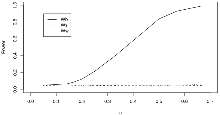
Processes generated by Case 1 are considered to shed light on the control of the Type I errors of the studied tests. The results are reported inTable 1. On the other hand, processes generated by Case 2 are considered for the power study. The results are given inTable 2andFigure 1. Note that inTable 1andTable 2we takea =1.1,b=11, andc=0.5, while inFigure 1we take several values forcanda=1.1,b=11.
In our example the studied tests seem to control the Type I errors reasonably well (seeTable 1). We can remark that the standard test provides satisfactory results. Nevertheless, this out-come does not have to be generalized since we have seen in Section2that the standard test is in general inadequate in pres-ence of time-varying variance. Now if we turn to the alternative given by Case 2, Table 2clearly shows that the standardWst
and WhiteWwtests have no power as the sample sizes increase
on the contrary of the bootstrap Wb test. For instance theWb
test is almost always rejecting the null hypothesisH0for sam-ple sizesT =1000, while theWstandWwtests are completely
not able to detect the alternative in this case. This confirms the theoretical results obtained when0112(r)dr≈0.
In the above power experiments the changes of12(r) around zero were fixed by a constant c. In this part we illustrate the ability of the tests to detect departures from the null hypothesis 12(r)
=0, while we again have0112(r)dr
=0 but taking several values forc(Figure 1). Here the sample is fixedT =500.
Table 1. The empirical size for the studied tests with asymptotic nominal level 1%, 5%, 10% anda=1.1,b=11,c=0.5
Asymptotic nominal level
1% 5% 10%
Wst Ww Wb Wst Ww Wb Wst Ww Wb
Sample size 50 0.010 0.007 0.007 0.048 0.050 0.047 0.102 0.113 0.105 100 0.009 0.009 0.010 0.057 0.066 0.066 0.095 0.096 0.107 200 0.011 0.010 0.011 0.045 0.047 0.052 0.101 0.116 0.122 500 0.011 0.010 0.010 0.042 0.047 0.050 0.099 0.101 0.101 1000 0.008 0.009 0.010 0.056 0.051 0.051 0.088 0.097 0.103
Table 2. The empirical power for the studied tests based on asymptotic nominal levels 1%, 5%, 10% anda=1.1,b=11,c=0.5
Asymptotic nominal level
1% 5% 10%
Wst Ww Wb Wst Ww Wb Wst Ww Wb
Sample size 50 0.014 0.005 0.003 0.056 0.040 0.045 0.110 0.085 0.132 100 0.012 0.005 0.012 0.056 0.038 0.102 0.098 0.079 0.213 200 0.017 0.010 0.076 0.063 0.048 0.305 0.106 0.093 0.512 500 0.011 0.006 0.486 0.050 0.038 0.837 0.105 0.080 0.930 1000 0.015 0.011 0.966 0.056 0.045 0.997 0.108 0.088 1.000
We clearly observe that the relative rejection frequencies of the Wbtest increase when the covariance structure12(r)=0 goes
away from zero but with0112(r)dr
=0. On the other hand we again remark that the relative rejection frequencies of the tests based on the assumption of constant variance remain close to the asymptotic nominal level even whenctakes large values.
4.2 Application to Macroeconomic Datasets
In this part we compare theWstandWwtests with theWbtest
by investigating instantaneous causality relationships in U.S. macroeconomic datasets.
4.2.1 Money Supply and Inflation in the United States. The relationship between money supply and inflation is fundamental in the macroeconomic theories for explaining the influence of monetary policy on economy. For instance, the quantity theory of money assumes a proportional relationship between money supply and the price level. The reader is referred to Case, Fair, and Oster (2011) or Mankiw and Taylor (2006) concerning the theoretical links which can be made between money supply and inflation. Many studies investigate this relation from an empir-ical point of view. Their results are, however, ambiguous. For instance, Turnovsky and Wohar (1984) used a simple macro model to investigate the relationship and find that the rate of in-flation is independent of the monetary growth rate in the United States over the period 1923–1960, while Benderly and Zwick
(1985) or Jones and Uri (1987) gave some evidence of a rela-tionship over the respective periods 1955–1982 and 1953–1984. Here we investigate the hypothesis of an instantaneous causal relationship between money supply and inflation in the United States over the period 1979–1995.
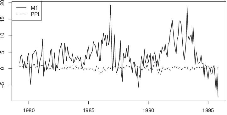
The data considered here are the M1 money stock (M1) and the Producer Price Index for all commodities (PPIACO). The M1 represents the money supply and PPIACOthe inflation from the point of view of producers. The M1 index is provided by the Board of Governors of the Federal Reserve System while the PPIACO index is provided by the U.S. Department of Labor. The data are taken from 04/1979 to 12/1995 with a monthly frequency. The length of the series is T =200. The data are available on the web site of the Federal Reserve Bank of St. Louis (Series ID : M1 and PPIACO). Their first differences denoted byM1 andPPIACOare plotted inFigure 2.
We adjusted a VAR(1) model to the first differences of the series. The autoregressive order is chosen by using portmanteau tests adapted to the framework of VAR processes with time-varying covariance (see Patilea and Ra¨ıssi 2013 for details). The outcomes inTable 3suggest that the model is well fitted. The estimation of the model by the OLS method is given in Table 4.
The residuals of the VAR(1) estimation are next recovered to test the null hypothesis of constant unconditional residual vari-ance. A corrected Inclan-Tiao test proposed by Sans´o, Arag´o,
0.0 0.1 0.2 0.3 0.4 0.5 0.6 0.7
0.0
0.2
0.4
0.6
0.8
1.0
c
Po
w
e
r
Wb Ws Ww
Figure 1. The empirical power of theWb,Wst, andWwtests for fixed sample sizeT =500 and varyingcparameter. The asymptotic nominal level is 5% and we takea=1.1,b=11.
Giai Gianetto and Ra¨ıssi: Testing Instantaneous Causality in Presence of Nonconstant Unconditional Covariance 51
1980 1985 1990 1995
−5
0
5
10
15
20
M1 PPI
Figure 2. Evolution of the variationsM1 andPPIACO.
Table 3. Thep-values of the Box–Pierce test adapted to our nonstandard framework for checking the adequacy of the VAR(1)
model adjusted to the U.S. M1 and inflation data
Number of lags
3 6 12
BPOLS 0.4384 [1.1198] 0.8169 [1.9071] 0.8165 [3.2870]
NOTE: The corresponding statistics are displayed into brackets. The BPOLScorresponds to
the portmanteau test based on the OLS proxies of theut’s.
and Carrion (2004) is used for this purpose. It is based on the following statistic:
κ =sup
k
|Ck−kσˆ2|
T( ˆη4−σˆ4) ,
whereCk =kt=1(ut−u¯)2, ˆσ2=T−1CT and ˆη4=T−1kt=1 (ut−u¯)4withutthe studied residuals. Under the null hypothesis
of constant unconditional variance errors and ifut is iid with
E[(ut−u¯)4]<+∞, the asymptotic distribution of the test is
given by
κ ⇒sup
r |
W∗(r)|,
whereW∗(r)=W(r)−rW(1) is a Brownian bridge andW(r) is a standard Brownian motion. The values of theκstatistic are 1.219 and 1.214 for the two residuals components of the VAR(1) model, while the critical values at the significance level of 10% and 5% are, respectively, 1.167 and 1.3 (seeTable 1in Sans´o, Arag´o, and Carrion2004). Let us recall that our bootstrapWb
Table 4. The OLS estimators of the matrixA01(see Equation (2.1))
for theVAR(1) model adjusted to the U.S. M1 and inflation data
A01
0.643 [0.064] −1.124 [0.360] −0.009 [0.007] 0.439 [0.102]
NOTE: Standard deviations of the parameters are displayed in brackets.
test is valid whatever the behavior of the unconditional residual variance contrary to the standardWstand WhiteWwtests.
Next, the tests studied in this article are implemented. Note that we used 399 bootstrap iterations for the bootstrapWbtest.
From Table 5 we see that thep-value of the Wb test is quite
different from those of the standardWst and White Ww tests.
For instance the null hypothesis of no instantaneous causality is rejected by the Wb test for a significance level of 10% on
the contrary to the other tests. These observations can be ex-plained by the covariance structure of the innovations. Indeed the nonparametric estimation of this covariance structure plotted inFigure 3shows that12(r) seems not null over the considered period while its seems that0112(r)dr ≈0.
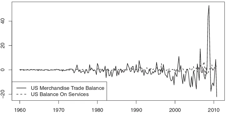
4.2.2 Merchandise Trade Balance and Balance on Services in the United States. The merchandise trade balance and the balance on services can be seen as indicators of the economic health of a country. The U.S. merchandise trade balance is the account which redraws the value of the exported goods and the value of the imported goods. The U.S. balance on services is similarly the account which redraws the value of the ex-ported services and the value of the imex-ported services. Here, we search to quantify if it exists an instantaneous causality re-lation between these two macroeconomic indicators. The data are provided by the Bureau Analysis of the U.S. Department of Commerce and taken from 01/1960 to 01/2011 with quarterly frequency. The length of the series isT =204. They are avail-able on the web site of the Federal Reserve Bank of St. Louis (Series ID : BOPBM and BOPBSV).
Similarly to the first dataset, we consider the first differences of the data (see Figure 4). A VAR(2) model is adjusted to the data (estimation results not reported here). The adequacy
Table 5. Thep-values of theWst,Ww, andWbtests for testing instantaneous causality between the U.S. M1 and inflation data
Wst Ww Wb
p-values 0.268 [1.225] 0.201 [1.632] 0.058 [10.54]
NOTE: The corresponding test statistics are displayed in brackets.
0.0 0.2 0.4 0.6 0.8 1.0
−4
−3
−2
−1
0
r
Estimated co
v
ar
iance str
ucture
US M1−PPI
US Balance Goods−Services
Figure 3. The Nadaraya-Watson kernel estimation of the covariance structure12(r) for the two datasets. The estimator is defined as in
Patilea and Ra¨ıssi (2012) which showed that such estimator is consistent under A1 unless at the break points.
of the model is again checked using portmanteau tests which are valid in our framework. The portmanteau test suggests to choose a VAR(2) model. Indeed thep-value of the BPOLStest is 0.65[5.29] for five autocorrelations in the portmanteau statis-tics (the portmanteau statistic is given into brackets). Next the corrected Inclan-Tiao test proposed by Sans´o, Arag´o, and Car-rion (2004) is applied to the two residuals components of the VAR(2) estimation. Theκstatistics are 2.223 and 2.591 for the two residuals components while the corresponding critical value is 1.547 (seeTable 1in Sans´o, Arag´o, and Carrion2004). This allows to reject the null hypothesis of constant variance with a significant level of 1%.
Thep-values of the tests for instantaneous causality are next computed from the residuals as for the first dataset. The out-comes displayed inTable 6show that the tests have quite differ-ent results. In view of the nonconstant variance of the studied series (seeFigure 3), the result corresponding to theWb test is
more reliable.
Table 6. Thep-values of theWst,Ww, andWbtests for testing the instantaneous causality between the U.S. balance data
Wst Ww Wb
p-value 0.0498 [3.848] 0.341 [0.907] 0.441 [190.142]
NOTE: The corresponding test statistics are displayed in brackets.
5. CONCLUSION
This article studies the problem of testing instantaneous causality in the important case where the unconditional covari-ance is time-varying. We found that the Wald tests based on the assumption of constant unconditional covariance may have no power in this nonstandard framework. As a consequence, we propose bootstrap test for testing the instantaneous causality hypothesis when the unconditional covariance structure is time-varying. In particular this test is shown to be consistent, and we illustrate these theoretical results through a set of numerical
1960 1970 1980 1990 2000 2010
−20
0
20
40
US Merchandise Trade Balance US Balance On Services
Figure 4. Evolution of the first differences of the U.S. merchandise trade balance and the U.S. balance on services in billion of U.S. dollars.
Giai Gianetto and Ra¨ıssi: Testing Instantaneous Causality in Presence of Nonconstant Unconditional Covariance 53
experiments. We show that the tests based on the stationary as-sumption are outperformed by the bootstrap test. The outcomes obtained from macroeconomic datasets suggest that the classi-cal Wald tests may deliver results which are quite different from the bootstrap test.
SUPPLEMENTARY MATERIAL
The supplementary material contains the proof of Equation (3.1) and Proposition 1. Some numerical experiments are also provided for illustrating the effect of lag length selection in VAR models prior testing instantaneous causality.
[Received March 2013. Revised February 2014.]
REFERENCES
Amendola, A., and Francq, C. (2009), “Concepts and Tools for Nonlinear Time Series Modelling,” inHandbook of Computational Econometrics, eds. D. A. Belsley, and E. J. Kontoghiorghes, New York: Wiley, chapter 10. [46] Andrews, B., Davis, R. A., and Jay Breidt, F. (2006), “Maximum Likelihood
Estimation for All-Pass Time Series Models,”Journal of Multivariate Anal-ysis, 97, 1638–1659. [46]
Ashenfelter, O., and Card, D. (1982), “Time Series Representations of Economic Variables and Alternative Models of the Labour Market,”The Review of Economic Studies, 49, 761–782. [46]
Aue, A., H¨ormann, S., Horv´ath, L., and Reimherr, M. (2009), “Break Detection in the Covariance Structure of Multivariate Time Series Models,”The Annals of Statistics, 37, 4046–4087. [46,48]
Azrak, R., and Melard, G. (2006), “Asymptotic Properties of Quasi-Maximum Likelihood Estimators for Arma Models With Time-Dependent Coeffi-cients,”Statistical Inference for Stochastic Processes, 9, 279–330. [46] Bahadur, R. (1960), “Stochastic Comparison of Tests,”Annals of Mathematical
Statistics, 31, 276–295. [48]
Bai, J. (2000), “Vector Autoregressive Models With Structural Changes in Re-gression Coefficients and in Variance-Covariance Matrices,”Annals of Eco-nomics and Finance, 1, 303–339. [46]
Bauwens, L., Laurent, S., and Rombouts, J. V. (2006), “Multivariate Garch Models: A Survey,”Journal of Applied Econometrics, 21, 79–109. [46] Benderly, J., and Zwick, B. (1985), “Inflation, Real Balances, Output, and
Real Stock Returns [Stock Returns, Real Activity, Inflation, and Money],” American Economic Review, 75, 1115–1123. [50]
Case, K., Fair, R., and Oster, S. (2011),Principles of Macroeconomics(10th ed), Upper Saddle River, NJ: Prentice Hall. [50]
Dahlhaus, R. (1997), “Fitting Time Series Models to Nonstationary Processes,” The Annals of Statistics, 25, 1–37. [46,47]
Dahlhaus, R., and Rao, S. S. (2006), “Statistical Inference for Time-Varying Arch Processes,”The Annals of Statistics, 34, 1075–1114. [46]
Davidson, R., and Flachaire, E. (2008), “The Wild Bootstrap, Tamed at Last,” Journal of Econometrics, 146, 162–169. [48]
Den Haan, W., and Levin, A. (1997), “A Practitioner’s Guide to Robust Covari-ance Matrix Estimation,” inHandbook of Statistics 15: Robust Inference, eds. G. Maddala, and C. Rao, Amsterdam: Elsevier, pp. 299–342. [46,47] Engle, R. F., and Rangel, J. G. (2008), “The Spline-Garch Model for
Low-Frequency Volatility and Its Global Macroeconomic Causes,”Review of Financial Studies, 21, 1187–1222. [46]
Francq, C., and Gautier, A. (2004), “Estimation of Time-Varying Arma Models With Markovian Changes in Regime,”Statistics and Probability Letters, 70, 243–251. [46]
Gonc¸alvez, S., and Kilian, L. (2004), “Bootstrapping Autoregressions With Con-ditional Heteroskedasticity of Unknown Form,”Journal of Econometrics, 123, 89–120. [47,48]
——— (2007), “Asymptotic and Bootstrap Inference for AR (∞) Processes With Conditional Heteroskedasticity,”Econometric Reviews, 26, 609–641. [48]
Granger, C. (1969), “Investigating Causal Relations by Econometric Models and Cross-Spectral Methods,”Econometrica, 37, 424–438. [46]
Hafner, C., and Linton, O. (2010), “Efficient Estimation of a Multivariate Mul-tiplicative Volatility Model,”Journal of Econometrics, 159, 55–73. [46] Hamilton, J. (1983), “Oil and the Macroeconomy Since World War II,”Journal
of Political Economy, 91, 228–248. [46]
Hamori, S., and Tokihisa, A. (1997), “Testing for a Unit Root in the Presence of a Variance Shift,”Economics Letters, 57, 245–253. [46]
Hansen, B. (1995), “Regression With Nonstationary Volatility,”Econometrica, 63, 1113–1132. [46]
Hiemstra, C., and Jones, J. (1994), “Testing for Linear and Nonlinear Granger Causality in the Stock Price-Volume Relation,” Journal of Finance, 49, 1639–1664. [46]
Horowitz, J. L., Lobato, I. N., Nankervis, J. C., and Savin, N. E. (2006), “Boot-strapping the Box–Pierceq-Test: A Robust Test of Uncorrelatedness,” Jour-nal of Econometrics, 133, 841–862. [47]
Horv`ath, L., Kokoszka, P., and Zhang, A. (2006), “Monitoring Constancy of Variance in Conditionally Heteroskedastic Time Series,”Econometric The-ory, 22, 373–402. [46]
Inoue, A., and Kilian, L. (2002), “Bootstrapping Autoregressive Processes With Possible Unit Roots,”Econometrica, 70, 377–391. [47,48]
Jones, J., and Uri, N. (1987), “Money, Inflation and Causality (Another Look at the Empirical Evidence for the USA, 1953–84),”Applied Economics, 19, 619–634. [50]
Kim, C., and Park, J. (2010), “Cointegrating Regressions With Time Hetero-geneity,”Econometric Reviews, 29, 397–438. [46]
Kokoszka, P., and Leipus, R. (2000), “Change-Point Estimation in Arch Mod-els,”Bernoulli, 6, 513–539. [46]
Lee, B.-S. (1992), “Causal Relations Among Stock Returns, Interest Rates, Real Activity, and Inflation,”Journal of Finance, 47, 1591–1603. [46] Li, X., and Zhao, Z. (2013), “Testing for Changes in Autocovariances of
Non-parametric Time Series Models,”Journal of Statistical Planning and Infer-ence, 143, 237–250. [46]
L¨utkepohl, H. (2005), New Introduction to Multiple Time Series Analysis, Berlin: Springer. [46,47]
L¨utkepohl, H., and Kr¨atzig, M. (2004), Applied Time Series Econometrics, Cambridge: Cambridge University Press. [46]
Mankiw, G., and Taylor, M. (2006),Economics, Hampshire, UK: Cengage Learning EMEA. [50]
McConnell, M., and Perez-Quiros, G. (2000), “Output Fluctuations in the United States: What has Changed Since the Early 1980’s?”The American Economic Review, 90, 1464–1476. [46]
Patilea, V., and Ra¨ıssi, H. (2012), “Adaptive Estimation of Vector Autoregres-sive Models With Time-Varying Variance: Application to Testing Linear Causality in Mean,”Journal of Statistical Planning and Inference, 142, 2891–2912. [46,52]
——— (2013), “Corrected Portmanteau Tests for Var Models With Time-Varying Variance,”Journal of Multivariate Analysis, 116, 190–207. [50] Pesaran, M., and Timmermann, A. (2004), “How Costly is It to Ignore Breaks
When Forecasting the Direction of a Time Series?”International Journal of Forecasting, 20, 411–425. [46]
Qu, Z., and Perron, P. (2007), “Estimating and Testing Structural Changes in Multivariate Regressions,”Econometrica, 75, 459–502. [46]
Ramey, V., and Vine, D. (2006), “Declining Volatility in the U.S. Automobile Industry,”The American Economic Review, 96, 1876–1889. [46] Robinson, P. M. (1987), “Asymptotically Efficient Estimation in the
Pres-ence of Heteroskedasticity of Unknown Form,” Econometrica, 55, 875–891. [46]
Sans´o, A., Arag´o, V., and Carrion, J. (2004), “Testing for Changes in the Un-conditional Variance of Financial Time Series,”Revista de Econom´ıa Fi-nanciera, 4, 32–53. [46,51]
Sensier, M., and Van Dijk, D. (2004), “Testing for Volatility Changes in U.S. Macroeconomic Time Series,”The Review of Economics and Statistics, 86, 833–839. [46]
Sims, C. (1972), “Money, Income, and Causality,”The American Economic Review, 62, 540–552. [46]
St˘aric˘a, C. (2004), “Is Garch (1, 1) as Good a Model as the Nobel Prize Ac-colades Would Imply?” Technical Report RePEc:wpa:wuwpem:0411015, EconWPA. [46]
Tsay, R. (1988), “Outliers, Level Shifts, and Variance Changes in Time Series,” Journal of Forecasting, 7, 1–20. [46]
Turnovsky, S. J., and Wohar, M. E. (1984), “Monetarism and the Aggregate Economy: Some Longer-Run Evidence,”The Review of Economics and Statistics, 66, 619–629. [50]
White, H. (1980), “A Heteroskedasticity-Consistent Covariance Matrix Estima-tor and a Direct Test for Heteroskedasticity,”Econometrica, 48, 817–838. [46]
Wu, F. (1986), “Jackknife, Bootstrap and Other Resampling Methods in Re-gression Analysis,”The Annals of Statistics, 14, 1261–1295. [47] Wu, W. B. (2007), “Strong Invariance Principles for Dependent Random
Vari-ables,”Annals of Probability, 35, 2294–2320. [46]
Xu, K., and Phillips, P. (2008), “Adaptive Estimation of Autoregressive Mod-els With Time-Varying Variances,”Journal of Econometrics, 142, 265– 280. [46]
Zhao, Z., and Li, X. (2013), “Inference for Modulated Stationary Processes,” Bernoulli, 19, 205–227. [46]