Full Terms & Conditions of access and use can be found at
http://www.tandfonline.com/action/journalInformation?journalCode=ubes20
Download by: [Universitas Maritim Raja Ali Haji] Date: 11 January 2016, At: 19:30
Journal of Business & Economic Statistics
ISSN: 0735-0015 (Print) 1537-2707 (Online) Journal homepage: http://www.tandfonline.com/loi/ubes20
Interest Rates and Money in the Measurement of
Monetary Policy
Michael T. Belongia & Peter N. Ireland
To cite this article: Michael T. Belongia & Peter N. Ireland (2015) Interest Rates and Money in the Measurement of Monetary Policy, Journal of Business & Economic Statistics, 33:2, 255-269, DOI: 10.1080/07350015.2014.946132
To link to this article: http://dx.doi.org/10.1080/07350015.2014.946132
Accepted author version posted online: 31 Jul 2014.
Submit your article to this journal
Article views: 381
View related articles
View Crossmark data
Interest Rates and Money in the Measurement
of Monetary Policy
Michael T. B
ELONGIADepartment of Economics, University of Mississippi, University, MS 38677([email protected])
Peter N. I
RELANDDepartment of Economics, Boston College, Chestnut Hill, MA 02467 ([email protected])
Over the last 25 years, a set of influential studies has placed interest rates at the heart of analyses that interpret and evaluate monetary policies. In light of this work, the Federal Reserve’s recent policy of “quantitative easing,” with its goal of affecting the supply of liquid assets, appears to be a radical break from standard practice. Alternatively, one could posit that the monetary aggregates, when measured properly, never lost their ability to explain aggregate fluctuations and, for this reason, represent an important omission from standard models and policy discussions. In this context, the new policy initiatives can be characterized simply as conventional attempts to increase money growth. This view is supported by evidence that superlative (Divisia) measures of money often help in forecasting movements in key macroeconomic variables. Moreover, the statistical fit of a structural vector autoregression deteriorates significantly if such measures of money are excluded when identifying monetary policy shocks. These results cast doubt on the adequacy of conventional models that focus on interest rates alone. They also highlight that all monetary disturbances have an important “quantitative” component, which is captured by movements in a properly measured monetary aggregate.
KEY WORDS: Divisia money; Monetary policy shocks; Quantitative easing.
1. INTRODUCTION
More than 25 years ago, Bernanke and Blinder (1988)
com-pactly summarized the choice facing a central bank. After mod-ifying a standard, Keynesian IS curve to account for shocks to the financial sector, their analysis reached two clear and straight-forward conclusions:
“But suppose the demand for money increases (line 2), which sends a contractionary impulse to GNP. Since this shock raises M, a monetarist central bank would contract reserves in an effort to stabilize money, which would destabilize GNP. This, of course, is the familiar Achilles heel of monetarism. Notice, however, that this same shock would make credit contract. So a central bank trying to stabilize credit would expand reserves. In this case, a credit-based policy is superior to a money-based policy.
The opposite is true, however, when there are credit-demand shocks. Line 4 tells us that a contractionary (for GNP) credit-demand shock lowers the money supply but raises credit. Hence a monetarist central bank would turn expansionary, as it should, while a creditist central bank would turn contractionary, which it should not.
We therefore reach a conclusion similar to that reached in discussing indicators: If money-demand shocks are more im-portant than credit-demand shocks, then a policy of targeting credit is probably better than a policy of targeting money.” (p. 438)
The authors then investigated whether the demand for money or credit was relatively more stable and found evidence to con-clude that the demand for credit, especially since 1980, was more stable; the implication was that, on the basis of this evi-dence, monetary policy would have better success in stabilizing Gross National Product (GNP) if it stabilized credit rather than variations in money.
The question posed by Bernanke and Blinder in 1988 was important then and, in view of the large shocks to credit
de-mand that have occurred since 2007, it still is correct to ask a similar question of central banks today: If the stabilization of nominal spending (which encompasses the Federal Reserve’s dual mandate of goals for price stability and real output) is to be achieved, which intermediate targeting strategy will accomplish this most effectively? The modern literature, however, contains relatively little of this discussion. Instead, the intervening years have narrowed the focus almost entirely to interest rate rules of
the type proposed by Taylor (1993) or some alternative guide to
setting the federal funds rate. The monetary aggregates have all but disappeared from the discussion.
In what follows, we briefly review the context in which the original Bernanke and Blinder article was written and the events that led to scuttling monetary aggregates both from mod-ern mainstream models and, by extension, from discussions of policy options. We then offer some counter-arguments to this consensus that suggest the role of the aggregates, as informa-tion variables or intermediate targets may have been mistakenly closed. With this as backdrop, we propose that the Federal Re-serve’s recent “experiments” with “quantitative easing” might usefully be viewed not as a radical break from the past necessi-tated by the zero lower bound on the federal funds rate, but as an extension of policies that have led, systematically, to move-ments in monetary aggregates that have been followed, first, by movements in real Gross Domestic Product (GDP) and, later, by movements in nominal prices. This real-world experiment illustrates both the dangers of a monetary policy strategy that focuses solely on targeting interest rates and the limitations of
© 2015American Statistical Association Journal of Business & Economic Statistics
April 2015, Vol. 33, No. 2 DOI:10.1080/07350015.2014.946132
255
an intellectual framework that fails to account for the important role that always has, and still is, played by variations in the growth rate of the aggregate quantity of money.
2. HISTORICAL CONTEXT
When Bernanke and Blinder (1988) appeared, the debate
about choosing money or the federal funds rate as an intermedi-ate target was anything but closed. Only a year after this article was published, the working paper (1989) version of Hallman, Porter, and Small (1991) outlined their influential P-star model, which linked M2 to the price level and had explicit Quantity
Theory foundations (Hallman, Porter, and Small1989).
More-over, only recently, both Meltzer (1987) and McCallum (1988)
presented monetary policy rules that used the monetary base to control variations in nominal spending directly. Conversely, the Federal Reserve officially abandoned its practice of monetary targeting in October 1982 and, since that time, has implemented monetary policy with a variety of approaches to targeting the federal funds rate. Dissension about the reliability of the signals given by the aggregates also had begun to grow, based in part on (faulty) predictions of renewed inflation in the mid-1980s that were supposed to have followed the rapid growth of M1 that had been observed. Because some of the most prominent economists had been embarrassed publicly when their warnings of
accel-erating inflation never materialized (see, e.g., Friedman1984,
1985), cracks in the empirical foundations of monetarism had
been revealed; Nelson (2007, pp. 162–168) and Barnett (2012,
pp. 107–111) offer discussions of the role that money supply measurement played in this episode.
These cracks grew larger when several key articles were
pub-lished in the early 1990s. First, Friedman and Kuttner (1992)
presented evidence indicating that the strong association be-tween money and aggregate economic activity appeared to be an artifact of two decades: The 1960s and 1970s. If the estima-tion period for the same relaestima-tionships contained data from the 1980s, the authors found that previously strong associations be-tween money and aggregate spending were no longer significant and that the demand for money function exhibited instability. The same article also found that money’s explanatory power was replaced by variations in short-term interest rates, includ-ing the 4–6 month commercial paper rate, the 3-month Treasury bill rate, and the spread between the two. Several months later,
Bernanke and Blinder (1992) reinforced these findings by
ex-amining the role of the federal funds rate in the monetary trans-mission mechanism. Like Friedman and Kuttner, these authors found that any role for money was minimized once the federal funds rate was introduced into the empirical framework. The conclusion was that any association money might have had with aggregate activity prior to 1980 had been seriously, and perhaps irredeemably, undermined by the financial innovations era.
The empirical evidence supporting this perspective accumu-lated on two fronts throughout the 1990s. One line of investiga-tion found that previously stable demand for money funcinvestiga-tions now exhibited considerable instability and, in doing so, violated a basic condition necessary for any reliance on the monetary ag-gregates as intermediate targets or indicator variables. A branch of this research found consistently that variations in the federal funds rate and the commercial paper Treasury bill rate spread
both were closely linked to the cycle. In combination, the break-downs in what had been strong associations between money and nominal magnitudes and the growing body of evidence linking interest rates to aggregate activity shifted the focus of research and monetary policy to models that had the federal funds rate at their core. Taylor’s (1993) influential article reinforced this shift in emphasis by showing how well the Federal Reserve had adjusted its federal funds rate target in response to move-ments in output and inflation during the late 1980s and early 1990s. By the end of the decade, the mainstream macro model
outlined by Clarida, Gali, and Gertler (1999) included an
equa-tion for the federal funds rate but not the aggregate quantity of money. In this “New Keynesian” model, as Eggertsson and
Woodford (2003) emphasized, the thrust of monetary policy—
expansionary or contractionary—gets summarized entirely by current and expected future short-term nominal interest rates.
Our first set of empirical findings suggests, however, that this conventional wisdom may have been built on the basis of re-sults that are not entirely robust. Related arguments have been made before. For instance, Thoma and Gray (1998) pointed to the importance of outliers in the data from 1974 in driving
the results in Friedman and Kuttner (1992) and Bernanke and
Blinder (1992) that link interest rates to economic activity. In
addition, both Belongia (1996) and Hendrickson (2011) have
replicated various portions of Friedman and Kuttner (1992) by
doing nothing more than replacing the Federal Reserve’s offi-cial simple sum measures of money with superlative (Divisia) indexes of money. After estimating the same relationships over the same sample periods with only this change, these authors found that money still shares a strong relationship with aggre-gate economic activity and that the demand for money function still exhibits stability. Because simple sum indexes cannot in-ternalize pure substitution effects, as emphasized by Barnett
(1980, 2012) and Belongia and Ireland (2012a), the Federal
Reserve’s official money supply data incorporate measurement error of unknown magnitude in their construction that will in-fluence economic inference. Our results add to this evidence by finding that when Divisia measures of money are included in the place of their simple sum counterparts, these quantity measures contain information and possess significant explanatory power comparable to that found in interest rates.
We derive a second set of results by incorporating Divisia measures of money into a structural vector autoregression (struc-tural VAR or SVAR) similar to that developed by Leeper and
Roush (2003). Our framework shows how the use of Divisia
monetary aggregates allows for better measurement of the key variables, as well as a more theoretically appealing depiction of the demand for monetary services; both assist in the crucial task of disentangling money supply from money demand. We find, as do Leeper and Roush, that including measures of money in the SVAR’s information set helps reduce the so-called “price puz-zle,” according to which an identified, contractionary monetary policy shock is associated initially with a rise in the aggregate level of prices. More important, we show that specifications that depict monetary policy as following a standard Taylor-type rule are rejected, statistically, in favor of an alternative that assigns a key role to the monetary aggregates; we find that, by contrast, restricting the policy equation to focus even more specifically on money does very little damage to the model’s empirical fit.
We also find, by making use of valuable new data on the Divisia aggregates provided by the Center for Financial Stability (CFS) and described by Barnett et al. (2013), that our results are ro-bust to the level of monetary aggregation. Finally, we use the structural VAR to gauge the effects of Federal Reserve policy in the years leading up to and immediately following the finan-cial crisis of 2007 and 2008; strikingly, these results corroborate
Barnett’s (2012) arguments that monetary instability looms as
an important factor in recent U.S. monetary history. Our results also provide a rationale for at least some aspects of the Fed’s moves toward “quantitative easing.”
Throughout our analysis and discussion, we take care to avoid dogmatic interpretations of our results. Our message certainly is not that interest rates play no role in the process through which monetary policy actions are transmitted through the economy. Instead, we wish to emphasize the important disconnect that appears between our empirical results (as well as those of Leeper
and Roush2003), pointing to a significant role for money, and
the recent theoretical literature, which focuses largely if not exclusively on interest rates instead. Understanding where the information content of the monetary aggregates comes from, and how it can be efficiently exploited in the design of monetary policy, remains as important today as it was a quarter century
ago, when Bernanke and Blinder’s (1988) work appeared.
3. THE INFORMATION CONTENT OF INTEREST RATES AND MONEY
Bernanke and Blinder (1992) examined the relative
informa-tion content of money and interest rates in explaining variainforma-tions in assorted measures of real activity in the context of an equation of this form:
whereYt is one of several measures of real activity to be
ex-plained,Xt is a measure of monetary policy, Pt is the
Con-sumer Price Index, which adjusts each estimation for any effects from changes in the general price level,αandλi,βi, and γi,
i=1,2,. . . ,6, are regression coefficients, and six lags of each monthly variable appear on the right-hand side. Their measures of real activity ranged from capacity utilization and housing starts to several measures of labor market activity and retail sales. Bernanke and Blinder used the Federal Reserve’s simple sum measures of M1 and M2 as well as the federal funds rate, the Treasury bill rate, and the 30 year Treasury bond rate as
measures of “X” in the equation above.
In the interest of space and because our research question is directed to the effects of measurement on inferences about money’s effect on economic activity and to the relative influ-ences of monetary aggregates and the funds rate on real activity, we report here only a partial set of replications and extensions of the results from the original Bernanke and Blinder article. In particular, we limit our work to estimations with simple sum measures of M1 and M2 and the funds rate and add Divisia mea-sures of M1, M2, and MZM (M2, less small time deposits, plus Institution-only Money Market Mutual Funds) as described by Barnett et al. (2013). As discussed by Motley (1988), the Money,
Zero Maturity (MZM) aggregate limits itself to items that are immediately convertible, without penalty, to some form of a medium of exchange.
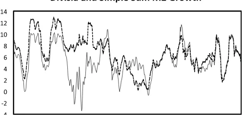
To help foreshadow the results we report below, Figure 1
compares the behavior of simple sum and Divisia measures of M2. The top panel shows year-over-year growth rates in both aggregates, to highlight cyclical movements while smoothing out higher frequency noise; the bottom panel plots the differ-ence between these series. Statistically, the differdiffer-ence variable
shown in the bottom panel has a nonzero mean equal to−1.25,
sizable standard deviation and first-order autocorrelation of 2.57
and 0.989, and negative skewness−1.07. Moreover, a standard
Augmented Dickey-Fuller test on the difference variable
indi-cates that this series is not stationary (−1.95 against a 0.05
critical value of−2.87). This result implies that a central bank attempting to achieve some nominal target by monitoring the growth rate of money eventually will drift off path by monitor-ing sum M2 rather than its Divisia counterpart.
A visual comparison of the simple sum and Divisia growth
rates shown inFigure 1points to the episode of disinflation and
financial deregulation of the early 1980s as the principal source of negative skewness, noted above, in the difference series. Dur-ing this period, the Divisia measure provides the stronger and more accurate signal of monetary tightness; the simple sum series dramatically overstates the true rate of money growth by failing to internalize the effects of portfolio shifts out of traditional, noninterest-bearing monetary assets, and into newly
Figure 1. Divisia versus simple sum M2 growth. The top panel shows year-over-year percentage growth rates of the Center for Finan-cial Stability’s Divisia M2 aggregate (thick solid line) and the Federal Reserve’s official simple sum M2 aggregate (thin dashed line). The bottom panel plots the difference between the two growth rate series.
Table 1. Causality test results: sample period 1967.01–1979.09
Forecasted variable Simple sum M1 Simple sum M2 Federal funds Divisia M1 Divisia M2 Divisia MZM
Industrial production 0.193 0.024 0.034 0.308 0.041 0.042
Capacity utilization 0.186 0.052 0.013 0.292 0.124 0.095
Employment 0.493 0.233 0.109 0.619 0.136 0.067
Unemployment rate 0.152 0.276 0.105 0.215 0.177 0.068
Housing starts 0.435 0.020 0.030 0.373 0.063 0.153
Personal income 0.000 0.017 0.044 0.000 0.003 0.003
Retail sales 0.006 0.133 0.009 0.010 0.504 0.617
Consumption 0.137 0.486 0.045 0.225 0.788 0.871
Durable goods orders 0.045 0.017 0.008 0.046 0.032 0.019
NOTES: Values are marginal significance levels for the coefficients on the monetary policy variable “X” included in the regression Equation (1). Values in bold indicate significance at the 5% level.
created, but somewhat less liquid, interest-earning accounts such as monetary market mutual funds and deposit accounts.
Fried-man’s (1984,1985) predictions of a return to higher inflation
during this episode were based, primarily, on his observations of robust growth in the simple sum monetary aggregates; hence,
these graphs support Barnett’s (2012) contention that Friedman
might have reached different conclusions had he monitored data on the Divisia aggregates instead.
The series inFigure 1also show that especially over the period since 1985, Divisia M2 has grown at a rate that consistently exceeds the growth rate of the simple sum M2 during periods of falling interest rates, particularly during the early stages of the 1990–1991, 2001, and 2007–2009 recessions; conversely, Divisia M2 growth tends to fall short of simple sum growth during periods of rising interest rates. Belongia and Ireland (2012a) used a New Keynesian model to show, theoretically, how liquidity effects such as these, manifesting themselves in an inverse relationship between money growth and interest rates, show up much more clearly in Divisia monetary aggregates than in their simple sum counterparts. Consistent with these theoretical results and the reduced-form correlations implied
by the series shown in Figure 1, the SVAR we develop and
estimate below associates monetary policy easings that lower nominal interest rates with strongly accelerating rates of Divisia money growth and, conversely, monetary tightenings that raise nominal interest rates with sharp contractions in Divisia money growth.
With six measures of how monetary policy might influence alternative indicators of real activity, we were left with choices
about sample periods for the model’s estimation. In a perfect world, we would have been able to replicate all of the samples in the original Bernanke and Blinder work but this is not possible because the Divisia data originate in January 1967 and the first sample for the original study began in 1959. We can terminate our samples, however, in 1979.12 and 1989.12 as was the case in the original work and, in the spirit of examining the robust-ness of the results, we can reestimate the same relationships on data drawn completely beyond the terminal date of the original study. In all, Bernanke and Blinder’s causality tests are repeated
across six samples and the results are reported in Tables1–6;
the entries in the tables are marginal significance levels. In each case, we are interested in two questions. First, do differences in measurement between simple sum and Divisia aggregation indicate important cases where money, when measured by one of the Federal Reserve’s official aggregates, shows no effect on economic activity, yet is linked to economic activity by a Di-visia measure? Second, are DiDi-visia measures of money and the funds rate linked to economic activity in different ways across alternative measures of economic activity and sample periods? We now turn to the results for answers to these questions.
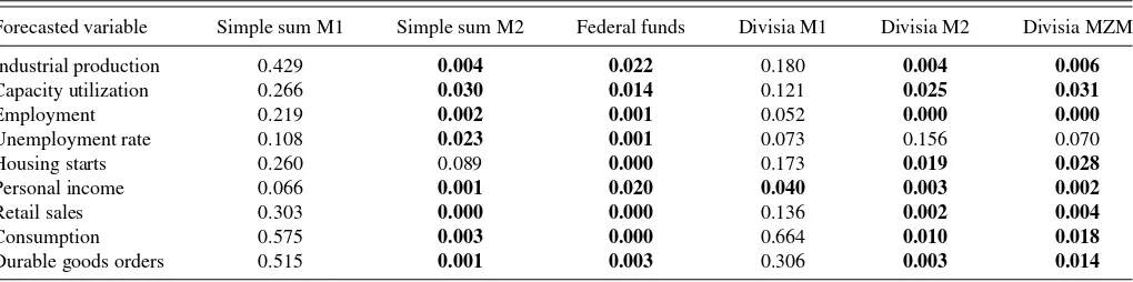
The first two tables report results for samples that resem-ble most closely those employed in the original Bernanke and Blinder study; although the beginning date now is 1967.01, the terminal dates are 1979.09 (to coincide with the beginning of the Federal Reserve’s announced plan to target money growth) and 1989.12. As noted above, each entry in these tables corresponds to the significance level for the statistic testing the hypothesis
that all lags of the monetary variable “X” can be excluded from
Table 2. Causality test results: sample period 1967.01–1989.12
Forecasted variable Simple sum M1 Simple sum M2 Federal funds Divisia M1 Divisia M2 Divisia MZM
Industrial production 0.429 0.004 0.022 0.180 0.004 0.006
Capacity utilization 0.266 0.030 0.014 0.121 0.025 0.031
Employment 0.219 0.002 0.001 0.052 0.000 0.000
Unemployment rate 0.108 0.023 0.001 0.073 0.156 0.070
Housing starts 0.260 0.089 0.000 0.173 0.019 0.028
Personal income 0.066 0.001 0.020 0.040 0.003 0.002
Retail sales 0.303 0.000 0.000 0.136 0.002 0.004
Consumption 0.575 0.003 0.000 0.664 0.010 0.018
Durable goods orders 0.515 0.001 0.003 0.306 0.003 0.014
NOTE: See notes to Table 1.
Table 3. Causality test results: sample period 1975.04–1989.12
Forecasted variable Simple sum M1 Simple sum M2 Federal funds Divisia M1 Divisia M2 Divisia MZM
Industrial production 0.043 0.059 0.022 0.030 0.006 0.005
Capacity utilization 0.044 0.141 0.009 0.020 0.015 0.013
Employment 0.019 0.018 0.004 0.014 0.003 0.002
Unemployment rate 0.044 0.010 0.001 0.029 0.030 0.035
Housing starts 0.767 0.507 0.002 0.550 0.198 0.102
Personal income 0.090 0.000 0.030 0.074 0.037 0.009
Retail sales 0.367 0.005 0.025 0.146 0.108 0.039
Consumption 0.830 0.091 0.031 0.747 0.502 0.487
Durable goods orders 0.485 0.611 0.005 0.444 0.123 0.161
NOTE: See notes to Table 1.
Table 4. Causality test results: sample period 1990.01–2007.12
Forecasted variable Simple sum M1 Simple sum M2 Federal funds Divisia M1 Divisia M2 Divisia MZM
Industrial production 0.424 0.690 0.016 0.381 0.891 0.943
Capacity utilization 0.147 0.514 0.006 0.294 0.672 0.725
Employment 0.796 0.816 0.736 0.532 0.946 0.892
Unemployment rate 0.005 0.009 0.014 0.014 0.038 0.047
Housing starts 0.373 0.677 0.002 0.007 0.290 0.081
Personal income 0.778 0.509 0.428 0.676 0.579 0.533
Retail sales 0.000 0.007 0.104 0.000 0.003 0.001
Consumption 0.000 0.025 0.307 0.000 0.021 0.002
Durable goods orders 0.010 0.094 0.000 0.253 0.201 0.226
NOTE: See notes to Table 1.
Table 5. Causality test results: sample period 1975.04–2007.12
Forecasted variable Simple sum M1 Simple sum M2 Federal funds Divisia M1 Divisia M2 Divisia MZM
Industrial production 0.129 0.968 0.005 0.004 0.093 0.037
Capacity utilization 0.013 0.371 0.002 0.132 0.156 0.213
Employment 0.215 0.744 0.001 0.014 0.059 0.030
Unemployment rate 0.253 0.174 0.000 0.067 0.302 0.180
Housing starts 0.416 0.221 0.000 0.009 0.004 0.002
Personal income 0.585 0.406 0.178 0.036 0.185 0.081
Retail sales 0.031 0.586 0.046 0.002 0.150 0.024
Consumption 0.426 0.669 0.188 0.075 0.328 0.194
Durable goods orders 0.025 0.398 0.000 0.004 0.014 0.027
NOTE: See notes to Table 1.
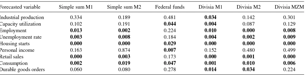
Table 6. Causality test results: sample period 2000.01–2013.12
Forecasted variable Simple sum M1 Simple sum M2 Federal funds Divisia M1 Divisia M2 Divisia MZM
Industrial production 0.334 0.189 0.481 0.034 0.142 0.301
Capacity utilization 0.102 0.191 0.044 0.004 0.087 0.129
Employment 0.013 0.002 0.224 0.010 0.000 0.008
Unemployment rate 0.003 0.008 0.184 0.004 0.002 0.009
Housing starts 0.000 0.000 0.029 0.000 0.000 0.000
Personal income 0.163 0.874 0.007 0.152 0.480 0.499
Retail sales 0.000 0.003 0.173 0.000 0.001 0.000
Consumption 0.002 0.019 0.047 0.001 0.010 0.006
Durable goods orders 0.060 0.080 0.278 0.014 0.034 0.224
NOTE: See notes to Table 1.
the regression Equation (1); smaller values, therefore, point to a stronger role for the monetary policy measure. The results both confirm and reject the findings of original work in several ways. First, as in the original article, the funds rate is shown to have a significant effect on all measures of economic activ-ity but two. Unlike the original article when M2 affected only retail sales and M1 had no marginal significance on any vari-able, the results here show that simple sum measures of money, especially M2, have effects on multiple measures of economic activity. It is unknown whether these differing results can be attributed to differences in vintages of data, a change in the starting date for the estimation, or issues associated with
repli-cating the original work as discussed in Thoma and Gray (1998,
footnote 2).
With respect to issues of measurement, however, the tables
also reveal some important consequences. In Table 1, for the
sample that terminates prior to the financial innovations era, there is little to distinguish, for example, sum and Divisia M1: Both have significant effects on personal income, retail sales, and durable goods orders. In the case of M2, the sum measure is significantly associated with four measures of real activity and the Divisia measure three, with a 0.06 significance level on a
fourth variable. InTable 2, however, which includes a sample
that terminates at 1989.12, the results reveal what was at stake when financial innovations induced substitutions among com-ponents of a monetary aggregate and those substitutions would have generated aberrant behavior in an index that could not in-ternalize pure substitution effects. Now, rather than diminishing the strength of any association between money and variations in real activity, the last two rows ofTable 2indicate that Divisia M2 and MZM are related to eight of the nine measures. And, while the funds rate is linked to all of the nine measures, these results hardly can be interpreted as evidence that money lost its ability to explain aggregate fluctuations after the 1970s. In fact, to emphasize the thrust of this article, the case that money is un-related to aggregate fluctuations depends entirely on the results in the table’s first column where the Federal Reserve’s simple sum measure of M1 fails to help forecast movements in all nine measures of real activity. Instead, as a general impression, the
results inTable 2for both broad Divisia aggregates are at odds
with the conclusions of the original Bernanke and Blinder article and, for that matter, work in the spirit of Friedman and Kuttner as well: Monetary aggregates—when measured properly—exhibit significant associations with a majority of the indicators of busi-ness cycle activity.
Because the first two samples include 1974, a period Thoma
and Gray (1998) found to include several interest rate outliers
that can influence standard inference,Table 3reports results us-ing an estimation period that covers 1975.04 through 1989.12. Although the federal funds rate remains associated with all nine measures of economic activity over this sample, both simple sum measures of money now appear related to four out of the nine indicators. The effects of money become stronger still when the Divisia aggregates are used: Divisia M1 is significantly as-sociated with four variables, Divisia M2 with five, and Divisia MZM with six. Particularly when the issue of measurement is considered, therefore, these results are sufficient to give one pause before abandoning the monetary aggregates as indicators of monetary policy.
Table 4reports results for a sample drawn from data com-pletely beyond the publication of the original study, 1990.01 through 2007.12, and they offer more evidence on the impor-tance of measurement. In this case, simple sum and Divisia M1 are both related to four of the variables, while simple sum and Divisia M2 and Divisia MZM are each related to three. The fed-eral funds rate significantly influences five of the nine variables but, with the exception of the unemployment rate, to different measures of activity than those closely connected to the mon-etary aggregates. Thus, if one is interested in the question, “Is money or the funds rate more closely linked to economic
ac-tivity?” the results inTable 4 indicate that it matters not only
how the quantity of money is measured but also on the
met-ric by which economic activity is measured. Likewise,Table 5
reports results from estimations across the 1975.04–2007.12 pe-riod, which abstracts from the interest rate outlier issue and ends prior to the beginning of the most recent economic downturn. Again, the funds rate relates significantly to many of the vari-ables, but so do the measures of money, particularly, in this case, Divisia M1 and MZM.
Finally,Table 6shows results from the period from 2000.01
through 2013.12, which includes the financial crisis and most re-cent recession, during and after which the Federal Reserve used several rounds of large-scale asset purchases—“quantitative easing”—in an effort to provide further monetary stimulus while its federal funds rate target was constrained by the zero lower bound. Notably, all six measures of monetary policy appear sig-nificantly related to subsequent movements in real consumption spending and housing starts, variables tied most directly to the crisis and its effects on American families. Throughout this lat-est episode, however, the Divisia measures of money appear most closely linked to movements in real economic activity, compared not only to the corresponding simple sum measures but also to the federal funds rate, which is significant in only four of nine cases.
The general message—that the loss of explanatory power for the monetary aggregates can be traced to the continued use of the Fed’s flawed simple sum aggregation methods—seems to be verified by the results in this table and the tables that
precede it. These results also present, as in Belongia (1996)
and Hendrickson (2011), additional cases in which an
ear-lier rejection of money’s influence can be reversed when the Federal Reserve’s simple sum aggregates are replaced by Di-visia aggregates in the same experiment. Over all, there is no evidence in these nonnested tests to conclude that the funds rate can be preferred to money—or vice versa—as an indica-tor or potential intermediate target for the conduct of monetary policy.
4. MEASURING MONETARY POLICY
To dig deeper into the sources of the links between money, interest rates, output, and prices, we follow Leeper and Roush
(2003), and build a structural vector autoregressive model for
these same variables. As a first step, we move from a monthly to a quarterly frequency for the data, which allows us to use
real GDP as our measure of aggregate outputYt and the GDP
deflator as our measure of the price levelPt. We use the federal
funds rate as a measure of the short-term nominal interest rate
Rt and one of the Divisia monetary aggregates to measure the
flow of monetary servicesMt.
To this list of variables we add two more. First, to assist in disentangling shocks to money supply from those to money
de-mand, we use the user-cost measureUt, also provided by Barnett
et al. (2013), that is the price dual to the Divisia monetary ag-gregateMt. Second, to mitigate the so-called “price puzzle” that
associates an exogenous monetary tightening with an initial rise instead of fall in the aggregate price level, we follow the
now-standard practice, first suggested by Sims (1992), and include
a measure of commodity prices PCt—the CRB/BLS spot index
compiled now by the Commodity Research Bureau (CRB) and earlier by the Bureau of Labor Statistics (BLS)—in the structural VAR. The beginning of the quarterly sample period, 1967.1, is dictated once again by the availability of the monetary statistics. To obtain our benchmark results, we end the sample after 2007.4 to avoid potential distortions associated with the most recent, severe recession; but later, we also consider results that obtain when the sample is extended through 2013.4. Again following conventions throughout the literature on structural VARs, out-put, prices, money, and commodity prices enter the model in log-levels, while the federal funds rate and the Divisia user-cost measures enter as decimals and in annualized terms, that is, a federal funds rate quoted as 5% on an annualized basis enters the dataset with a reading ofRtequal to 0.05.
Stacking the variables at each date into the 6 × 1 vector
Xt =[Pt Yt CPt Rt Mt Ut]′, (2)
the structural model takes the form
Xt =µ+
matrix of coefficients, andεt is a 6 × 1 vector of serially and
mutually uncorrelated structural disturbances, each following the standard normal distribution.
The reduced form associated with (3) is
Xt =µ+ q
j=1
jXt−j +xt, (4)
where the 6 × 1 vector of zero-mean disturbances
xt =[pt yt cpt rt mt ut]
′
(5)
is such thatExtxt′=.
Comparing (3) and (4) reveals that the structural and reduced-form disturbances are linked via
Axt=εt, (6)
whereA=B−1
andBB′=.
Since the covariance matrix
for the reduced-form innovations contains only 21 distinct ele-ments, at least 15 restrictions must be imposed on the elements
of the matrixB or its inverseAto identify the structural
dis-turbances from the information communicated by the reduced form.
A common approach to solving this identification problem
requiresAto be lower triangular. If the fourth element of the
vectorεt is interpreted as a monetary policy shock, this
identi-fication scheme assumes that the aggregate price level, output, and commodity prices respond with a lag to monetary policy actions, and that the Federal Reserve adjusts the federal funds rate contemporaneously in response to movements in the these same three variables but ignores the Divisia monetary aggre-gates and their user costs. Although recursive schemes like this one are based on assumptions about the timing of the responses of one variable to movements in the others, in this case one might also interpret the fourth line in the vector of equations from (6),
a41pt+a42yt+a43cpt+a44rt =εtmp, (7)
as an expanded version of the Taylor rule that includes com-modity prices as well as GDP and the GDP deflator among the variables that influence the Federal Reserve’s setting for its fed-eral funds rate target. Note, however, that this Taylor rule serves only to capture the contemporaneous co-movement between the variables in (7); interest rate smoothing, and any other system-atic responses of Federal Reserve policy to lagged data, will be reflected in the autoregressive coefficients in both (3) and (4). Likewise, the fifth line in (6),
a51pt+a52yt+a53cpt+a54rt+a55mt =εmdt (8)
might be interpreted as a flexibly specified money demand equa-tion, linking the demand for monetary services to the aggre-gate price level, aggreaggre-gate output, and the short-term nomi-nal interest rate, with the commodity-price variable entering as well.
An alternative approach to identification, followed by Leeper and Roush (2003), imposes restrictions in (6) so as to allow the money supply to enter into the description of the monetary policy rule and to provide a more tightly specified and theoretically consistent description of money demand. Leeper and Roush conducted their empirical analysis using the Federal Reserve’s simple sum M2 measure of the money supply; here, we modify and extend their approach to apply to Divisia measures of money instead. Our benchmark nonrecursive model parameterizes the
matrixAas
Only 19 free parameters enter into (9), implying that the
model satisfies the necessary conditions for recovering the struc-tural disturbances inεtfrom the reduced-form innovationsxtvia
(6). The first two rows in (9) indicate that in this specification, as in the recursive model described above, the price level and aggregate output are assumed to respond sluggishly, with a lag, to monetary disturbances. The absence of zero restrictions in the third row, however, reflects our preference for modeling commodity prices as an “information variable,” responding im-mediately to all of the shocks that hit the economy.
Row four of (9) continues to describe a generalized
Tay-lor rule, but one in which the supply of monetary services, as opposed to commodity prices, enters as an additional
variable:
a41pt+a42yt+a44rt+a45mt =εmpt , (10)
whereεtmprepresents the identified monetary policy shock.
Ire-land (2001) embedded a monetary policy of this general form
into a New Keynesian model. One interpretation of this rule is that it depicts the Federal Reserve as adjusting its federal funds rate target in response to changes in the money supply, as well as in response to movements in aggregate prices and output. An alternative interpretation is that (10) describes Federal Reserve policy actions as impacting simultaneously on both interest rates and the money supply. Simultaneity of this kind will arise, quite naturally, even when Federal Reserve officials themselves pay no explicit attention to simple sum or Divisia monetary aggre-gates if, for example, the open market operations they conduct to implement changes in their federal funds rate target also have implications for the behavior of the monetary aggregates, which then turn out to be important for describing the effects that those policy actions have on the economy. With monetary services now appearing in the policy rule, it is worth recalling
that Taylor’s (1979) original specification was based on money
rather than interest rates; our rule in (10), therefore, combines elements from both this earlier specification and Taylor’s (1993) now much more celebrated rule for the funds rate.
Row five, meanwhile, links the demand for real monetary services to aggregate output as a scale variable and to the user cost, or price dual, associated with the Divisia quantity aggregate:
a52yt+a55(mt−pt)+a56ut=εmdt . (11)
Belongia (2006) discussed why money demand relationships
of this form are more coherent than more commonly used speci-fications, like (8), that use a nominal interest rate in its place. The reason for this preferred specification is that economic aggrega-tion theory provides not only a guide to measuring the quantity of money more accurately, but it also provides, in the dual to the quantity measure, the true “price” of monetary services.
Finally, row six of (9),
a64rt+a65(mt−pt)+a66ut=εmst (12)
summarizes the behavior of the private financial institutions that, together with the Federal Reserve, create liquid assets that provide households and firms with monetary services. Belongia
and Ireland (2012a) and Ireland (2012) modeled this behavior
in more detail, to show how an increase in the federal funds rate, by increasing the cost at which banks acquire funds, gets passed along to the consumers of monetary services in the form of a
higher user cost; (12) adds the level of real monetary services
created as well, to allow for the possibility that banks’ costs may rise in the short run as they expand the scale of their operations. Thus, in (12),εms
t represents a shock to the monetary system
that makes it more difficult and expensive for private financial institutions to create liquid assets.
Compared to the recursive identification scheme described initially, the nonrecursive specification in (9) at once provides a more detailed and theoretically motivated description of the banks that supply monetary assets and the nonbank public that
demands those same assets. In addition, (9) permits the money
supply to enter into the description of Federal Reserve policy,
broadening the more conventional view that focuses on interest
rates alone. In fact, (9) also allows us to assess the adequacy
of this conventional view by comparing the empirical fit of our benchmark model to that of two more restrictive alternatives. In particular, when a45 =0 is imposed in (9), (10) collapses to a standard Taylor rule for adjusting the federal funds rate in response to movements in aggregate prices and output. On
the other hand, whena41 =0 anda42 =0 are imposed instead,
we obtain via (10) Leeper and Roush’s (2003) preferred
spec-ification, which places money much closer to center stage by identifying monetary policy shocks based solely on the inter-play between the money supply and interest rates; Leeper and
Zha (2003) and Sims and Zha (2006) also incorporated
money-interest rate rules of this simple form into structural vector au-toregressive models.
Since none of our alternative identification strategies imposes
any restrictions on the parameters in the vectorµof constant
terms or the matricesj,j =1, 2, . . ., q, of autoregressive
coefficients, these can be estimated efficiently by applying
or-dinary least squares to each equation in the reduced form (4).
For the recursive identification scheme in which the matrixA
is simply required to be lower-triangular, the usual approach
is followed, in which the matrixB in (3) is obtained through
the Cholesky factorization of the covariance matrix of the
reduced-form innovations. For the nonrecursive system (9) and
its two more highly constrained variants, the nonzero elements
of A are estimated via maximum likelihood as described by
Hamilton (1994, chap. 11, pp. 331–332). Throughout, the
pa-rameterqis set equal to 4, implying that 1 year of quarterly lags appear in the autoregression.
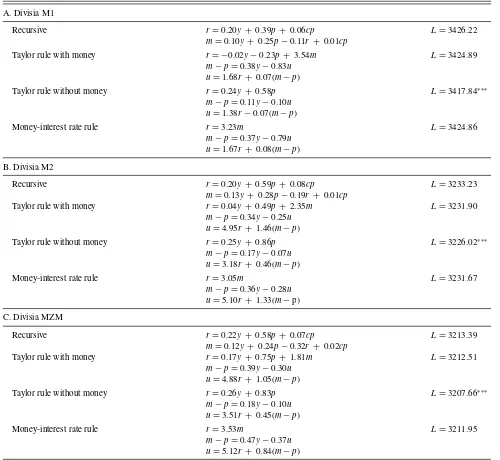
Table 7summarizes the results from estimating the vector au-toregression under each of the four identification schemes: the
recursive model, the structural model (9), and the two more
highly constrained versions of (9) just described. As noted
above, the quarterly sample period in each case begins in 1967.1
and runs through 2007.4. And while Table 7 focuses on
re-sults obtained with Divisia measures at the same three levels of aggregation—M1, M2, and MZM—used above to extend
Bernanke and Blinder’s (1992) analysis, additional tables from
the appendix to Belongia and Ireland (2012b) report the full
range of results derived with all of the other Divisia quantity
and user-cost series provided by Barnett et al. (2013) at the
Center for Financial Stability and as well as those reported by
Anderson and Jones (2011) at the St. Louis Federal Reserve
Bank.
To help prevent readers from getting lost in a forest of
num-bers, Table 7 displays estimates of the monetary policy and
money demand Equations (7) and(8) for the recursive model
and the monetary policy, money demand, and monetary system Equations (10)–(12) for the nonrecursive models. And to assist in their interpretations, each of these equations is renormalized to isolate, with a unitary coefficient, the interest rate on the left-hand side of the monetary policy equation, real monetary services on the left-hand side of the money demand equation, and the user cost of the monetary aggregate on the left-hand side of the monetary services equation. In this way, across all specifications and levels of monetary aggregation, the estimated coefficients can be seen at a glance to have, with few exceptions, the “correct” signs.
Table 7. Maximum likelihood estimates of structural vector autoregressions
A. Divisia M1
Recursive r=0.20y + 0.39p+ 0.06cp L=3426.22
m=0.10y+ 0.25p−0.11r + 0.01cp
Taylor rule with money r= −0.02y−0.23p+ 3.54m L=3424.89
m−p=0.38y−0.83u
u=1.68r + 0.07(m−p)
Taylor rule without money r=0.24y + 0.58p L=3417.84∗ ∗ ∗
m−p=0.11y−0.10u
u=1.38r−0.07(m−p)
Money-interest rate rule r=3.23m L=3424.86
m−p=0.37y−0.79u
u=1.67r + 0.08(m−p)
B. Divisia M2
Recursive r=0.20y + 0.59p+ 0.08cp L=3233.23
m=0.13y+ 0.28p−0.19r + 0.01cp
Taylor rule with money r=0.04y + 0.49p+ 2.35m L=3231.90
m−p=0.34y−0.25u
u=4.95r + 1.46(m−p)
Taylor rule without money r=0.25y + 0.86p L=3226.02∗ ∗ ∗
m−p=0.17y−0.07u
u=3.18r + 0.46(m−p)
Money-interest rate rule r=3.05m L=3231.67
m−p=0.36y−0.28u
u=5.10r + 1.33(m−p)
C. Divisia MZM
Recursive r=0.22y + 0.58p+ 0.07cp L=3213.39
m=0.12y+ 0.24p−0.32r + 0.02cp
Taylor rule with money r=0.17y + 0.75p+ 1.81m L=3212.51
m−p=0.39y−0.30u
u=4.88r + 1.05(m−p)
Taylor rule without money r=0.26y + 0.83p L=3207.66∗ ∗ ∗
m−p=0.18y−0.10u
u=3.51r + 0.45(m−p)
Money-interest rate rule r=3.53m L=3211.95
m−p=0.47y−0.37u
u=5.12r + 0.84(m−p)
NOTES: Each panel shows the estimates of Equations (7) and (8) from the recursive specification or Equations (10)–(12) from the nonrecursive models, together with the maximized value of the log-likelihood functionL.∗ ∗ ∗denotes that the null hypothesis that money can be excluded from the monetary policy rule is rejected at the 99% confidence level. In no case can the null hypothesis that the monetary policy rule includes money and interest rates alone be rejected in favor of the alternative that monetary policy follows the Taylor rule with money.
In particular, the Taylor-type monetary policy rules show the Federal Reserve increasing the federal funds rate in response to upward movements in output and prices, while the most par-simonious money-interest rate rule associates a contractionary monetary policy shock, that is, a positive realization forεtmp,
as one that simultaneously decreases the money supply and increases the funds rate. The money demand equations draw positive relationships between real money services and output as the scale variable and negative relationships between real money and the associated opportunity cost variable, be it the interest rate in the recursive model or the Divisia price dual in the nonrecursive frameworks. And in each of the nonrecursive
models, the estimates of (12) show how the private monetary
system passes increases in the federal funds rate along to con-sumers of monetary services in the form of higher user costs; these estimates also draw a positive association between real
monetary services and the user costs, consistent with our inter-pretation of this relationship as a “supply curve” for monetary services.
Compared to the most flexible nonrecursive model that in-cludes the monetary aggregate together with output and prices in the monetary policy Equation (10), the version that reverts to a more conventional Taylor rule by excluding money imposes a single constraint on the model. Therefore, this restriction can be tested by comparing two times the difference between the values of maximized log-likelihood functions across the two specifications to the critical values implied by a chi-squared distribution with one degree of freedom. Likewise, the restric-tions that exclude prices and output so that money and
inter-est rates alone appear in (10) can be tested by comparing two
times the difference in log-likelihoods to the critical values of a chi-squared distribution with two degrees of freedom. Quite
strikingly, across all three levels of monetary aggregation, the constraint excluding money from the monetary policy rule is rejected at the 99% confidence level while, in the meantime, the constraints excluding prices and output from the policy rule are imposed without any significant deterioration in the model’s statistical fit. As a matter of fact, the constraints imposed by the model with the most parsimonious money-interest rate rule cannot be rejected, even when the fit of this model is compared to the most flexible, recursive specification.
This first set of results reinforces those presented by Leeper
and Roush (2003) and casts doubt on the adequacy of
conven-tional descriptions of monetary policy that focus on interest rates alone. These results also join with those from Belongia
(1996) and Hendrickson (2011) by suggesting that perennial
debates about the “right” level of monetary aggregation, like
several other “unsolved problems” in monetary economics, re-flect more than any other factor an unfortunate reliance on sim-ple sum aggregates in previous empirical work. So long as one
accepts Barnett’s (1980) argument that economic aggregation
theory ought to be applied to measure the aggregate supply of monetary services just as it is applied to measure GDP, indus-trial production, or any other index of macroeconomic activity, one remains free to choose any monetary aggregate from M1
through MZM in drawing the main message fromTable 7: that
money does seem to matter, importantly, in describing the ef-fects of Federal Reserve policy.
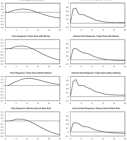
Figure 2, meanwhile, reveals another problem that emerges from the recursive specification and, as well, from the con-strained version of the nonrecursive model that also excludes money from the monetary policy rule. This figure displays
Figure 2. Impulse responses to monetary policy shocks. Each panel shows the response, in percentage points, of the price level or the interest rate to a one-standard-deviation monetary policy shock, derived under one of the four identification schemes described in the text. In each case, money is measured by the CFS’s Divisia MZM monetary aggregate.
impulse responses of the price level and the federal funds rate to monetary policy shocks, as identified by each of our four al-ternative strategies. The figure shows the results obtained using the Divisia MZM index of monetary services, but once again similar findings emerge when any of the other Divisia aggre-gates is employed instead. Even though the commodity price variable is included in all of the models, and even though the recursive model allows commodity prices to enter into the mon-etary policy Equation (7), this specification still gives rise to a
noticeable price puzzle. Here, as in Leeper and Roush (2003),
including money in the policy rule helps minimize the rise in prices that follows a contractionary policy shock. And strik-ingly, here, the price puzzle is greatly magnified in the third
row ofFigure 2, when money is excluded from the Taylor-type
interest rate rule, but is minimized in the last row, which uses
the simplest money-interest rate rule instead. In this last case, as well, the larger disinflationary effects shown in the left-hand column are associated with the smaller rise in the interest rate shown on the right.
All of these results provide reasons to prefer our most par-simonious description of a monetary policy shock as one that leads to a contraction in the quantity of money and a simultane-ous “liquidity effect” on interest rates. This specification cannot be rejected in favor of a more flexible alternative that includes prices and output in the policy rule and also produces identi-fied monetary policy shocks that most reliably associate tighter policy with falling prices.
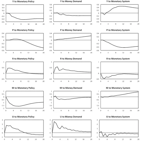
Figure 3, therefore, goes on to plot the impulse responses of output, prices, interest rates, and the quantity and user cost indexes for money to all three of the structural disturbances
Figure 3. Impulse responses. Each panel shows the response, in percentage points, of the indicated variable to the indicated one-standard-deviation shock, as implied by the structural VAR with the money-interest rate rule. Money is measured by the CFS’s Divisia MZM monetary aggregate.
appearing in Equations (10)–(12)—to monetary policy, to money demand, and to the private financial sector—implied by the constrained, nonrecursive model with the money-interest rate rule. Once more, the results shown use Divisia MZM as the measure of money, though very similar results obtain at all other
levels of aggregation. The first column ofFigure 3reveals that
the fall in prices and rise in the interest rate shown inFigure 2
that follow an identified monetary policy shock get accompanied by persistent declines in real GDP and the quantity of money. The increase in the federal funds rate works, as well, to increase
the user cost of money; Belongia and Ireland (2006) showed
that, through inflation-tax effects, a response in the own-price of money of exactly this kind transmits monetary policy shocks to output even in a model with completely flexible prices and wages.
The center column ofFigure 3shows impulse responses to
money demand shocks. The fall in output and rise in the in-terest rate associated with a shock that, on impact, increases the demand for monetary services are consistent with theory. And while the increase in the price level is counterintuitive,
Leeper and Roush (2003) presented an example where
aggre-gate prices do rise following a positive shock to money demand. Their example is based on Ireland’s (2001) version of the New Keynesian model in which the monetary policy rule also incor-porates money as well as the interest rate. More difficult to ex-plain is why, after the initial increase reflecting the shock itself, the quantity of monetary services falls persistently in figure’s fourth row; this finding calls for a more detailed investigation of money demand dynamics using the newly available series on the Divisia aggregates.
The right-hand column inFigure 3shows that a positive
real-ization of the shockεms
t that enters into Equation (12) describing
the behavior of the private financial sector generates a small ini-tial decline in output and a much larger and more persistent decrease in prices. A persistent fall in the nominal interest rate, perhaps reflecting a deliberate, systematic monetary policy re-sponse to the financial-sector disturbance, allows the user cost of money to decline and reverse the initial decline in the
quan-tity of monetary services. The panels inFigure 4examine, in
various ways, the same model’s interpretation of U.S. monetary policy over the sample period. The top panel simply plots the realizations of the monetary policy shockεmpt ; since (3) normal-izes each structural disturbance to have a standard deviation of one, the graph’s scale conveniently measures the size of each realized shock in standard deviations. Reassuringly, a series of large contractionary (positive) monetary policy shocks stand out during the period beginning in the fourth quarter of 1979 and continuing through the first quarter of 1982. Elsewhere in the sample, strings of large expansionary (negative) shocks appear from 1973.4 through 1974.4 and over an even longer period of time from 2001.1 through 2004.2.
The bottom two panels ofFigure 4show how the serially
un-correlated monetary policy shocks are translated, via the model’s autoregressive structure, into persistent movements, first in
out-put and then, with a lag, aggregate prices; Laidler (1997, pp.
1217–1219) described how dynamics like those shown here, in Figure 4, and previously, inFigure 3, are consistent with “buffer-stock” models of individuals’ money demand. Each of the graphs in these two panels plots the percentage-point
differ-Figure 4. Monetary policy shocks and their effects. The top panel plots the serially uncorrelated monetary policy shock from structural VAR with the money-interest rate rule, estimated with data from 1967.1 through 2007.4. Money is measured by the CFS’s Divisia MZM mon-etary aggregate. The bottom two panels plot the cumulative effects of these shocks on output and prices, as percentage-point differences be-tween the actual value of each variable at each date minus the value that, according to the estimated VAR, would have obtained in the absence of monetary policy shocks over the entire sample.
ence between the actual level of output or the aggregate price level and the level of the same variable implied by the model when all of estimated historical shocks except the monetary
pol-icy shocks are fed through (3). Therefore, each panel shows how
much higher or lower output or prices actually were at each date, compared the levels that would have prevailed, counterfactually, in the absence of monetary policy shocks.
The bottom panel ofFigure 4highlights, in particular, how
ac-commodative monetary policy shocks worked to increase prices by a total of 3 percentage points in the late 1970s and early 1980s. Interestingly, while the contractionary shocks in the early
1980s worked to halt temporarily this upward movement, the cumulative effect of monetary policy shocks contributed to re-newed price pressures in the late 1980s and early 1990s. Mone-tary policy was disinflationary throughout the 1990s, but the series of expansionary shocks realized during and after the 2001 recession contributed to rising prices starting in 2002.4 and continuing through 2005.4. Of course, the swings in prices
shown in Figure 4 represent only a fraction of those
ob-served over the entire sample period, indicating that our struc-tural VAR, like those estimated previously by Leeper and
Roush (2003), Primiceri (2005), and Sims and Zha (2006),
attributes the bulk of inflation’s rise and fall before and after 1980 not to monetary policy shocks but instead to the Fed-eral Reserve’s systematic response to other shocks that hit the economy.
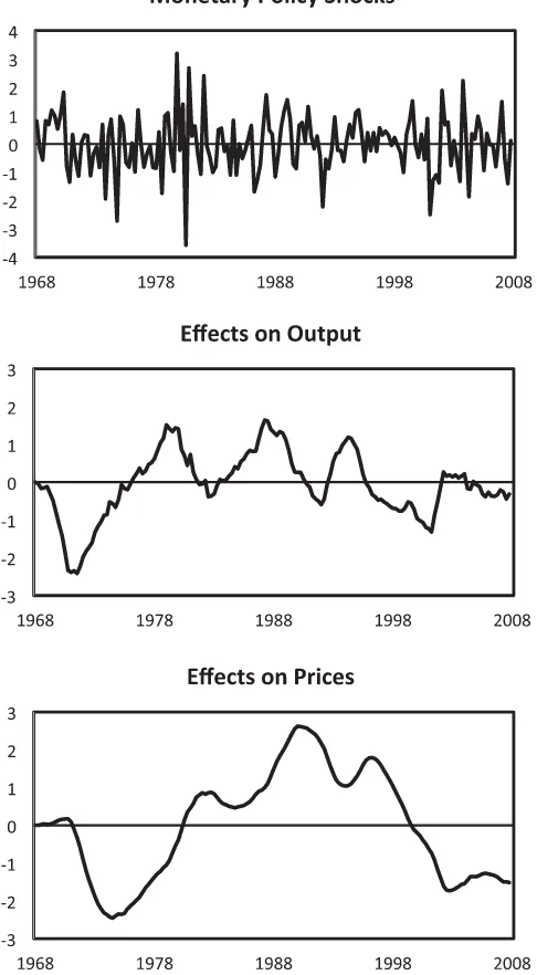
Finally,Figure 5displays the model’s implications when it
is reestimated with data running through 2013.4, still using the Divisia MZM aggregate and our preferred money-interest rate rule. To focus on monetary policy and its effects in the period just before, during, and after the financial crisis and severe recession, the series in the graphs begin in 2000.1, even though the data used to estimate the model continue to run all the way back to 1967.1. Strikingly, the monetary policy shocks shown in the top panel are largely contractionary from 2008.3 through 2010.2, consistent with findings from previous analyses by Hetzel (2009), Ireland (2011), Tatom (2011), and Barnett (2012), all of which point to overly restrictive monetary policy as, though perhaps not the principal cause of the “great recession,” at least an important factor contributing to its length and severity.
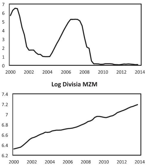
Figure 6helps in tracing these implications of the model back to original time series for interest rates and money. The top panel shows how the Federal Reserve lowered its federal funds rate target to a range between 0 and 0.25 percentage points in late 2008, where it has remained ever since. By itself, this unprece-dented policy action has been popularly interpreted as indicating that an extremely accommodative monetary policy has helped counteract the effects of the financial crisis on output both dur-ing and since the recession that began in 2007. The statistical results presented here, however, tell a much more detailed and nuanced story. Both the Granger causality test statistics shown inTable 6, which show strong forecasting power of the Divisia monetary aggregates for various measures of real activity, and the structural VAR, which depicts monetary policy actions as having effects on both interest rates and those same monetary aggregates, call special attention to the bottom panel ofFigure 6: For the period running from 2009.4 through 2010.2, the money stock displays—even more severe than a deceleration in its rate of growth—a sustained decline in its level.
In general, therefore, the dynamics shown inFigures 5and
6remind us of one of the principal lessons that Friedman and
Schwartz (1963) drew from their famous analysis of the Great
Depression of the 1930s, namely, that during a banking or fi-nancial crisis the demand for highly liquid assets may require a massive expansion of bank reserves simply to prevent broader measures of the money stock from declining. More
specifi-cally, the pattern of monetary shocks shown in Figure 5 and
the behavior of the money supply shown inFigure 6 suggest
strongly that the Federal Reserve pulled back too much, too
Figure 5. Monetary policy shocks and their effects. The top panel plots the serially uncorrelated monetary policy shock from structural VAR with the money-interest rate rule, estimated with data from 1967.1 through 2013.4. Money is measured by the CFS’s Divisia MZM mon-etary aggregate. The bottom two panels plot the cumulative effects of these shocks on output and prices, as percentage-point differences be-tween the actual value of each variable at each date minus the value that, according to the estimated VAR, would have obtained in the absence of monetary policy shocks over the entire sample.
soon, when it suspended its policies of quantitative easing during 2010.
On the other hand, the monetary shocks shown inFigure 5
be-come expansionary from 2010.3 through 2011.3, and the money
stock shown in Figure 6resumes its growth at the same time.
Our model, which assigns a key role to money in the policy rule, interprets every episode of monetary easing as “quantitative eas-ing” by associating them with increases in money growth and not simply declines in interest rates. It also confirms in particular that the Federal Reserve’s second round of bond purchases in 2010 and 2011 did have its intended expansionary effects. Thus,
the middle panel ofFigure 5shows that while monetary policy
Figure 6. Interest rates and the money stock. The top panel shows the effective federal funds rate and the second panel shows the log of the CFS’s Divisia MZM monetary aggregate; both series are quarterly and run from 2000.1 through 2013.4.
contributed to a cumulative decline in output of more than 2% from 2008.3 through 2010.4, it has been largely supportive of an accelerating recovery since then.
5. CONCLUSION
Our results call into question the conventional view that the stance of monetary policy can be described with exclusive refer-ence to its effects on interest rates and without consideration of simultaneous movements in the monetary aggregates. Whether by replicating and extending the results of a landmark study or by producing new results from a structural VAR, the message from Divisia monetary aggregates is that money always has had a significant role to play as an intermediate target or indicator variable and that any apparent deterioration in its information content can be traced to the measurement errors inherent in the practice of simple sum aggregation. These results also allow us to see the Federal Reserve’s recent policy of “quantitative eas-ing” in a new light: As having its intended stimulative effect by expanding the growth rate of a properly measured value of the money supply, over and above whatever effects it might have had by altering the shape of the yield curve.
Our results also highlight the disconnect between modern New Keynesian models, in which the quantity of money plays no special role once the time path for interest rates is accounted for. In working to bridge this divide, we suspect that researchers will be led to reconsider, as well, the same enduring questions
addressed by Bernanke and Blinder (1988) many years ago.
ACKNOWLEDGMENTS
The authors thank Rong Chen, Nicolas Groshenny, Josh Hen-drickson, David Laidler, Ed Nelson, and two anonymous ref-erees for extremely helpful comments on previous drafts and Richard Anderson, William Barnett, and Barry Jones for use-ful conversations and for their patience in answering questions about the construction of their series for the Divisia monetary aggregates. Dekuwmini Mornah provided able research assis-tance. Neither author received external support for, or has any financial interest that relates to, the research described in this article.
[Received September 2012. Revised May 2014.]
REFERENCES
Anderson, R. G., and Jones, B. E. (2011), “A Comprehensive Revision of the U.S. Monetary Services (Divisia) Indexes,”Federal Reserve Bank of St.
Louis Review, 93, 325–359. [262]
Barnett, W. A. (1980), “Economic Monetary Aggregates: An Application of Index Number and Aggregation Theory,”Journal of Econometrics, 14, 11– 48. [256,264]
——— (2012),Getting It Wrong: How Faulty Monetary Statistics Undermine
the Fed, the Financial System, and the Economy, Cambridge, MA: MIT
Press. [256,258,267]
Barnett, W. A., Liu, J., Mattson, R. S., and van den Noort, J. (2013), “The New CFS Divisia Monetary Aggregates: Design, Construction, and Data Sources,”Open Economies Review, 24, 101–124. [257,261,262]
Belongia, M. T. (1996), “Measurement Matters: Recent Results from Monetary Economics Reexamined,”Journal of Political Economy, 104, 1065–1083. [256,260,264]
——— (2006), “The Neglected Price Dual of Monetary Quantity Aggregates,”
inMoney, Measurement and Computation, eds. M. T. Belongia and J. M.
Binner, New York: Palgrave Macmillan. [262]
Belongia, M. T., and Ireland, P. N. (2006), “The Own-Price of Money and the Channels of Monetary Transmission,”Journal of Money, Credit, and
Banking, 38, 429–445. [266]
——— (2012a), “The Barnett Critique After Three Decades: A New Keyne-sian Analysis,” Working Paper No. 17885, National Bureau of Economic Research. [256,258,262]
——— (2012b), “Quantitative Easing: Interest Rates and Money in the Mea-surement of Monetary Policy,” Working Paper No. 801, Boston College, Department of Economics. [262]
Bernanke, B. S., and Blinder, A. S. (1988), “Credit, Money, and Aggregate Demand,”American Economic Review, 78, 435–439. [255,256,257,268] ——— (1992), “The Federal Funds Rate and the Channels of Monetary
Trans-mission,”American Economic Review, 92, 901–921. [256,257,262] Clarida, R., Gali, J., and Gertler, M. (1999), “The Science of Monetary Policy:
A New Keynesian Perspective,”Journal of Economic Literature, 37, 1661– 1707. [256]
Eggertsson, G. B., and Woodford, M. (2003), “The Zero Bound on Interest Rates and Optimal Monetary Policy,”Brookings Papers on Economic Activity, 139–211. [256]
Friedman, B. M., and Kuttner, K. N. (1992), “Money, Income, Price, and Interest Rates,”American Economic Review, 82, 472–492. [256]
Friedman, M. (1984), “Lessons from the 1979–82 Monetary Policy Experi-ment,”American Economic Review, 74, 397–400. [256,258]
——— (1985), “The Fed Hasn’t Changed Its Ways,”Wall Street Journal, 28. [256,258]
Friedman, M., and Schwartz, A. J. (1963),A Monetary History of the United
States,1867--1960, Princeton: Princeton University Press. [267]
Hallman, J. J., Porter, R. D., and Small, D. H. (1989), “M2 Per Unit of Potential GNP as an Anchor for the Price Level,” Staff Study 157, Washington, DC: Federal Reserve Board. [256]
——— (1991), “Is the Price Level Tied to the M2 Monetary Aggregate in the Long Run?,”American Economic Review, 81, 841–858. [256]
Hamilton, J. D. (1994),Time Series Analysis, Princeton: Princeton University Press. [262]
Hendrickson, J. (2011),Redundancy or Mismeasurement? A Reappraisal of
Money, Detroit: Wayne State University. [256,260,264]
Hetzel, R. L. (2009), “Monetary Policy in the 2008–2009 Recession,”Federal
Reserve Bank of Richmond Economic Quarterly, 95, 201–233. [267]