Full Terms & Conditions of access and use can be found at
http://www.tandfonline.com/action/journalInformation?journalCode=ubes20
Download by: [Universitas Maritim Raja Ali Haji] Date: 11 January 2016, At: 19:16
Journal of Business & Economic Statistics
ISSN: 0735-0015 (Print) 1537-2707 (Online) Journal homepage: http://www.tandfonline.com/loi/ubes20
Goodness of Fit: An Axiomatic Approach
Frank A. Cowell, Russell Davidson & Emmanuel Flachaire
To cite this article: Frank A. Cowell, Russell Davidson & Emmanuel Flachaire (2015) Goodness of Fit: An Axiomatic Approach, Journal of Business & Economic Statistics, 33:1, 54-67, DOI: 10.1080/07350015.2014.922470
To link to this article: http://dx.doi.org/10.1080/07350015.2014.922470
Accepted author version posted online: 21 May 2014.
Submit your article to this journal
Article views: 241
View related articles
Goodness of Fit: An Axiomatic Approach
Frank A. C
OWELLSTICERD, London School of Economics, Houghton Street, London WC2A 2AE, United Kingdom ([email protected])
Russell D
AVIDSONAMSE-GREQAM, Centre de la Vieille Charit ´e, 13236 Marseille, France and
Department of Economics; CIREQ, McGill University, Montreal, Quebec H3A 2T7, Canada ([email protected])
Emmanuel F
LACHAIREAix-Marseille Universit ´e, AMSE and IUF, Centre de la Vieille Charit ´e, 13236 Marseille, France ([email protected])
An axiomatic approach is used to develop a one-parameter family of measures of divergence between distributions. These measures can be used to perform goodness-of-fit tests with good statistical properties. Asymptotic theory shows that the test statistics have well-defined limiting distributions which are, however, analytically intractable. A parametric bootstrap procedure is proposed for implementation of the tests. The procedure is shown to work very well in a set of simulation experiments, and to compare favorably with other commonly used goodness-of-fit tests. By varying the parameter of the statistic, one can obtain infor-mation on how the distribution that generated a sample diverges from the target family of distributions when the true distribution does not belong to that family. An empirical application analyzes a U.K. income dataset.
KEY WORDS: Measures of divergence; Parametric bootstrap.
1. INTRODUCTION
In this article, we propose a one-parameter family of statistics that can be used to test whether an IID sample was drawn from a member of a parametric family of distributions. In this sense, the statistics can be used for a goodness-of-fit test. By varying the parameter of the family, a range of statistics is obtained and, when the null hypothesis that the observed data were indeed generated by a member of the family of distributions is false, the different statistics can provide valuable information about the nature of the divergence between the unknown true data-generating process (DGP) and the target family.
Many tests of goodness of fit exist already, of course. Test statistics, which are based on the empirical distribution function (EDF) of the sample, include the Anderson–Darling statistic (see Anderson and Darling 1952), the Cram´er–von Mises statistic, and the Kolmogorov–Smirnov statistic. See Stephens (1986) for much more information on these and other statistics. The Pearson chi-square goodness-of-fit statistic, on the other hand, is based on a histogram approximation to the density; a reference more recent than Pearson’s original article is Plackett (1983).
Here our aim is not just to add to the collection of exist-ing goodness-of-fit statistics. Our approach is to motivate the goodness-of-fit criterion in the same sort of way as is com-monly done with other measurement problems in economics and econometrics. As examples of the axiomatic method, see Sen (1976a) on national income, Sen (1976b) on poverty, and Ebert (1988) on inequality. The role of axiomatization is cen-tral. We invoke a relatively small number of axioms to capture the idea of divergence of one distribution from another using an informational structure that is common in studies of income mo-bility. From this divergence concept one immediately obtains a class of goodness-of-fit measures that inherit the principles
em-bodied in the axioms. As it happens, the measures in this class also have a natural and attractive interpretation in the context of income distribution. We emphasize, however, that the ap-proach is quite general, although in the sequel we use income distributions as our principal example.
To be used for testing purposes, the goodness-of-fit statistics should have a distribution under the null that is known or can be simulated. Asymptotic theory shows that the null distribution of the members of the family of statistics is independent of the parameter of the family, although that is certainly not true in finite samples. We show that the asymptotic distribution (as the sample size tends to infinity) exists, although it is not analyti-cally tractable. However, its existence serves as an asymptotic justification for the use of a parametric bootstrap procedure for inference.
A set of simulation experiments was designed to uncover the size and power properties of bootstrap tests based on our proposed family of statistics, and to compare these properties with those of four other commonly used goodness-of-fit tests. We find that our tests have superior performance. In addition, we analyze a U.K. dataset on households with below-average incomes, and show that we can derive a stronger conclusion by use of our tests than with the other commonly used goodness-of-fit tests.
The article is organized as follows. Section 2 sets out the formal framework and establishes a series of results that
© 2015American Statistical Association Journal of Business & Economic Statistics
January 2015, Vol. 33, No. 1 DOI:10.1080/07350015.2014.922470
Color versions of one or more of the figures in the article can be found online atwww.tandfonline.com/r/jbes.
54
characterize the required class of measures. Section3 derives the distribution of the members of this new class. Section4 ex-amines the performance of the goodness-of-fit criteria in prac-tice, and uses them to analyze a U.K. income dataset. Section5 concludes. All proofs are found in the Appendix.
2. AXIOMATIC FOUNDATION
The axiomatic approach developed in this section is in part motivated by its potential application to the analysis of income distributions.
2.1 Representation of the Problem
We adopt a structure that is often applied in the income-mobility literature. Let there be an ordered set of n income classes; each classi is associated with income levelxi where xi < xi+1,i=1,2, . . . , n−1. Letpi ≥0 be the size of class
i, i=1,2, . . . , n which could be an integer in the case of finite populations or a real number in the case of a contin-uum of persons. We will work with the associated cumulative mass ui =ij=1pj, i=1,2, . . . , n. The set of distributions is given by U :=u|u∈Rn
+, u1≤u2≤ · · · ≤un
. The ag-gregate discrepancy measurement problem can be character-ized as the relationship between two cumulative-mass vectors u,v∈U. An alternative equivalent approach is to work with z:=(z1, z2, . . . , zn), where eachzi is the ordered pair (ui, vi), i=1, . . . , nand belongs to a setZ, which we will take to be a connected subset ofR+×R+. The problem focuses on the
discrepancies between theu-values and thev-values. To cap-ture this we introduce a discrepancy functiond :Z→Rsuch thatd(zi) is strictly increasing in|ui−vi|. Write the vector of discrepancies as
d(z) :=(d(z1), . . . , d(zn)).
The problem can then be approached in two steps.
1. We represent the problem as one of characterizing a weak ordering1
on
Zn:=Z×Z× · · · ×Z
n
.
where, for any z,z′∈Znthe statement “z
z′” should be
read as “the pairs inz′ constitute at least as good a fit
ac-cording toas the pairs inz.” Fromwe may derive the antisymmetric part≻and symmetric part∼of the ordering.2 2. We use the function representingto generate an aggregate
discrepancy index.
In the first stage of Step 1 we introduce some properties for
, many of which correspond to those used in choice theory and in welfare economics.
1This implies that it has the minimal properties of completeness, reflexivity, and
transitivity.
2For any z,z′∈Zn “z≻z′” means “[zz′] & [z′z]”; and “z∼z′” means
“[zz′] & [z′z].”
2.2 Basic Structure
Axiom 1(Continuity). is continuous onZn.
Axiom 2 (Monotonicity). Ifz,z′∈Zn differ only in their ith
component thend(ui, vi)< d u′i, v′i
⇐⇒z≻z′.
For anyz∈Zndenote byz(ζ, i) the member ofZnformed by replacing theith component ofzbyζ ∈Z.
Axiom 3 (Independence). For z,z′∈Zn such that: z
∼z′
and zi =z′i for some i then z(ζ, i)∼z′(ζ, i) for all ζ ∈ [zi−1, zi+1]∩[z′i−1, z′i+1].
Ifzandz′are equivalent in terms of overall discrepancy and
the fit in classiis the same in the two cases then a local variation in componentisimultaneously inzandz′has no overall effect.
Axiom 4(Perfect local fit). Letz,z′∈Znbe such that, for some
iandj, and for someδ >0,ui =vi,uj =vj,u′i=ui+δ,vi′= vi+δ,u′j =uj −δ,v′j =vj −δand, for allk=i, j,u′k=uk, v′
k=vk. Thenz∼z′.
The principle states that if there is a perfect fit in two classes then movingu-mass andv-mass simultaneously from one class to the other has no effect on the overall discrepancy.
Theorem 1. Given Axioms 1 to 4,
(a) is representable by the continuous function given by
n
i=1
φi(zi),∀z∈Zn, (1)
where, for eachi=1, . . . , n,φi:Z→Ris a continu-ous function that is strictly increasing in|ui−vi|, with φ(0,0)=0; and
(b)
φi(u, u)=biu. (2)
Proof.In the Appendix.
Corollary 1. Sinceis an ordering it is also representable
by
φ
n
i=1
φi(zi)
, (3)
whereφiis defined as in (1), (2) andφ:R→Ris continuous and strictly increasing.
This additive structure means that we can proceed to evaluate the aggregate discrepancy problem one income class at a time. The following axiom imposes a very weak structural require-ment, namely that the ordering remains unchanged by some uniform scale change to both u-values and v-values simulta-neously. As Theorem 2 shows, it is enough to induce a rather specific structure on the function representing.
Axiom 5(Population scale irrelevance). For anyz,z′∈Znsuch
thatz∼z′,tz∼tz′for allt >0.
Theorem 2. Given Axioms 1 to 5is representable by
Proof.In the Appendix
The functionshi in Theorem 2 are arbitrary, and it is useful to impose more structure. This is done in Section2.3.
2.3 Mass Discrepancy and Goodness of Fit
We now focus on the way in which one compares the (u, v) discrepancies in different parts of the distribution. The form of (4) suggests that discrepancy should be characterized in terms of proportional differences:
This is the form for d that we will assume from this point onwards. We also introduce:
Axiom 6 (Discrepancy scale irrelevance). Suppose there are
z0,z′
The principle states this. Suppose we have two distributional fitsz0andz′
0that are regarded as equivalent under. Then scale
up (or down) all the mass discrepancies inz0andz′
0by the same
factort. The resulting pair of distributional fitszandz′will also
be equivalent.3
Theorem 3. Given Axioms 1 to 6is representable by
(z)=φ
Proof.In the Appendix.
2.4 Aggregate Discrepancy Index
Theorem 3 provides some of the essential structure of an aggregate discrepancy index. We can impose further structure by requiring that the index should be invariant to the scale of the u-distribution and to that of thev-distribution separately. In other words, we may say that the total mass in theu- and v-distributions is not relevant in the evaluation of discrepancy, but only the relative frequencies in each class. This implies that the discrepancy measure(z) must be homogeneous of degree zero in theui and in theviseparately. But it also means that the
3Also note that Axiom 6 can be stated equivalently by requiring that, for a given
z0,z′
0∈Znsuch thatz0∼z′0, either (a) anyzandz′ found by rescaling the
u-components will be equivalent or (b) anyzandz′found by rescaling the
v-components will be equivalent.
requirement thatφi is increasing in |ui−vi| holds only once the two scales have been fixed.
Theorem 4. If in addition to Axioms 1–6 we require that the
orderingshould be invariant to the scales of the massesui and of theviseparately, the ordering can be represented by
(z)=φ
Proof.In the Appendix.
A suitable cardinalization of (6) gives the aggregate discrep-ancy measure
The denominator ofα(α−1) is introduced so that the index, which otherwise would be zero forα=0 orα=1, takes on limiting forms, as follows forα=0 andα=1 respectively:
G0= −
Expressions (7)–(9) constitute afamilyof aggregate discrepancy measures where an individual family member is characterized by choice of α: a high positive α produces an index that is particularly sensitive to discrepancies wherevexceeds u and a negativeαyields an index that is sensitive to discrepancies whereuexceedsv. There is a natural extension to the case in which one is dealing with a continuous distribution on support Y ⊆R. Expressions (7)–(9) become, respectively:
1
Clearly there is a family resemblance to the Kullback and Leibler (1951) measure of relative entropy or divergence measure off2
fromf1
but with densitiesf replaced by cumulative distributionsF.
2.5 Goodness of Fit
Our approach to the goodness-of-fit problem is to use the index constructed in Section2.4to quantify the aggregate dis-crepancy between an empirical distribution and a model. Given a
set ofnobservations{x1, x2, . . . , xn}, the empirical distribution
where the order statisticx(i)denotes theith smallest observation,
and I is an indicator function such that I (S)=1 if statementS is true and I (S)=0 otherwise. Denote the proposed model distribution byF(·;θ), whereθis a set of parameters, and let
vi =F(x(i);θ), i=1, . . . , n
ui =Fnˆ (x(i))=
i
n, i=1, . . . , n.
Thenviis a set of nondecreasing population proportions gener-ated by the model from thenordered observations. As before, writeµvfor the mean value of thevi; observe that
µu= 1 α=1 we have, respectively, that
G0(F,Fnˆ )= −
the same distribution as the order statistics of a sample of sizendrawn from the uniform U(0,1) distribution. The statis-ticGα(F,Fˆn) in (10) is random only through theui, and so, for givenα andn, it has a fixed distribution, independent of F. Further, asn→ ∞, the distribution converges to a limiting distribution that does not depend onα.
Theorem 5. LetFbe a distribution function with continuous
positive derivative defined on a compact support, and let ˆFn be the empirical distribution of an IID sample of sizendrawn fromF. The statisticGα(F,Fnˆ ) in (10) tends in distribution as n→ ∞to the distribution of the random variable
1
whereB(t) is a standard Brownian bridge, that is, a Gaussian stochastic process defined on the interval [0,1] with covariance function
cov(B(t), B(s))=min(s, t)−st.
Proof.See the Appendix.
The denominator oftin the first integral in (11) may lead one to suppose that the integral may diverge with positive probabil-ity. However, notice that the expectation of the integral is
1
A longer calculation shows that the second moment of the inte-gral is also finite, so that the inteinte-gral is finite in mean square, and so also in probability. We conclude that the limiting distribution ofGαexists, is independent ofα, and is equal to the distribution of (11).
Remark.As one might expect from the presence of a
Brown-ian bridge in the asymptotic distribution ofGα(F,Fnˆ ), the proof of the theorem makes use of standard results from empirical pro-cess theory; see van der Vaart and Wellner (1996).
We now turn to the more interesting case in which Fdoes depend on a vectorθof parameters. The quantitiesvi are now given byvi=F(x(i),θˆ), where ˆθis assumed to be a root-n
con-sistent estimator of θ. If θ is the true parameter vector, then we can writexi =Q(ui, θ), whereQ(·, θ) is the quantile func-tion inverse to the distribufunc-tion funcfunc-tionF(·, θ), and theuihave the distribution of the uniform order statistics. Then we have vi=F(Q(ui, θ),θˆ), and
The statistic (10) becomes
Gα(F,Fnˆ )= α 1 respect toθ, and make the definition
P(θ)=
∞
−∞
p(x, θ) dF(x, θ).
Then we have:
Theorem 6. Consider a family of distribution functions
F(·, θ), indexed by a parameter vectorθ contained in a finite-dimensional parameter space. For eachθ∈, suppose that F(·, θ) has a continuous positive derivative defined on a compact support, and that it is continuously differentiable with respect to the vectorθ. Let ˆFnbe the EDF of an IID sample{x1, . . . , xn}of
sizendrawn from the distributionF(·, θ) for some given fixed θ. Suppose that ˆθis a root-nconsistent estimator ofθsuch that, asn→ ∞,
for some vector functionh, differentiable with respect to its first argument, and whereh(x, θ) has expectation zero whenxhas the distributionF(x, θ). The statisticGα(F,Fnˆ ) given by (12) has a finite limiting asymptotic distribution asn→ ∞, expressible as the distribution of the random variable
1
0
1 t
B(t)+p⊤(Q(t, θ), θ)
∞
−∞
h′(x, θ)B(F(x, θ)) dx
2
dt
−2
1
0
B(t) dt+P⊤(θ)
∞
−∞
h′(x, θ)B F(x, θ)dx
2
.
(14)
HereB(t) is a standard Brownian bridge, as in Theorem 5.
Proof.See the Appendix.
Remarks. The limiting distribution is once again independent
ofα.
The function h exists straightforwardly for most com-monly used estimators, including maximum likelihood and least squares.
So as to be sure that the integral in the first line of (14) con-verges with probability 1, we have to show that the nonrandom integrals
1
0
p(Q(t, θ), θ)
t dt and
1
0
p2(Q(t, θ), θ)
t dt
are finite. Observe that
1
0
p(Q(t, θ), θ)
t dt =
∞
−∞ p(x, θ)
F(x, θ)dF(x, θ)
=
∞
−∞
DθlogF(x, θ) dF(x, θ),
whereDθ is the operator that takes the gradient of its operand with respect toθ. Similarly,
1
0
p2(Q(t, θ), θ)
t dt =
∞
−∞
(DθlogF(x, θ))2
×F(x, θ) dF(x, θ).
Clearly, it is enough to require thatDθlog F(x, θ)should be bounded for allxin the support ofF(·, θ). It is worthy of note that this condition is not satisfied if varyingθcauses the support of the distribution to change.
In general, the limiting distribution given by (14) depends on the parameter vectorθ, and so, in general,Gαis not asymptot-ically pivotal with respect to the parametric family represented by the distributionsF(·, θ). However, if the family can be in-terpreted as a location-scale family, then it is not difficult to check that, if ˆθis the maximum-likelihood estimator, then even in finite samples, the statistic Gα does not in fact depend on θ. In addition, it turns out that the lognormal family also has this property. It would be interesting to see how common the property is, since, when it holds, the bootstrap benefits from an asymptotic refinement. But, even when it does not, the ex-istence of the asymptotic distribution provides an asymptotic justification for the bootstrap.
It may be useful to give the details here of the bootstrap pro-cedure used in the following section to perform goodness-of-fit tests, in the context both of simulations and of an application with real data. It is a parametric bootstrap procedure; see, for instance, Horowitz (1997) or Davidson and MacKinnon (2006). Estimates θ of the parameters of the family F(·, θ) are first obtained, preferably by maximum likelihood, after which the statistic of interest, which we denote by ˆτ, is computed, whether it is (10) for a chosen value ofαor one of the other statistics
studied in the next section. Bootstrap samples of the same size as the original data sample are drawn from the estimated distri-butionF(·,θˆ). Note that this isnota resampling procedure. For each of a suitable number Bof bootstrap samples, parameter estimatesθj∗,j =1, . . . , B, are obtained using the same esti-mation procedure as with the original data, and the bootstrap statisticτj∗computed, also exactly as with the original data, but withF(·, θj∗) as the target distribution. Then a bootstrapp-value is obtained as the proportion of theτj∗ that are more extreme than ˆτ, that is, greater than ˆτ for statistics like (10) which re-ject for large values. For well-known reasons—see Davison and Hinkley (1997) or Davidson and MacKinnon (2000)—the num-berBshould be chosen so that (B+1)/100 is an integer. In the sequel, we setB =999. This computation of thep-value can be used to test the fit of any parametric family of distributions.
4. SIMULATIONS AND APPLICATION
We now turn to the way the new class of goodness-of-fit statis-tics performs in practice. In this section, we first study the finite sample properties of ourGα test statistic and those of several standard measures: in particular we examine the comparative performance of the Anderson and Darling (1952) statistic (AD),
AD=n
∞
−∞
( ˆF(x)−F(x,θˆ))2 F(x,θˆ) 1−F(x,θˆ)
dF(x,θˆ),
the Cram´er-von-Mises statistic given by
CVM=n
∞
−∞ ˆ
F(x)−F(x,θˆ)2dF(x,θˆ),
the Kolmogorov–Smirnov statistic
KS=sup x |
ˆ
F(x)−F(x,θˆ)|,
and the Pearson chi-square (P) goodness-of-fit statistic
P=
m
i=1
(Oi−Ei)2/Ei,
where Oi is the observed number of observations in the ith histogram interval,Ei is the expected number in the ith his-togram interval and mis the number of histogram intervals.4 Then we provide an application using a U.K. dataset on income distribution.
4.1 Tests for Normality
Consider the application of theGα statistic to the problem of providing a test for normality. It is clear from expression (10) that different members of theGα family will be sensitive to different types of divergence of the EDF of the sample data from the modelF. We take as an example two cases in which the data come from a Beta distribution, and we attempt to test the hypothesis that the data are normally distributed.
4We use the standard tests as implemented with R; the number of intervalsmis
due to Moore (1986). Note that G, AD, CVM, and KS statistics are based on the empirical distribution function (EDF) and thePstatistic is based on the density function.
0.2 0.4 0.6 0.8 1.0
0.0
0.2
0.4
0.6
0.8
1.0
x
cum
ulativ
e distr
ib
ution function
Beta(5,2) Normal
0.0 0.2 0.4 0.6 0.8
0.0
0.2
0.4
0.6
0.8
1.0
x
cum
ulativ
e distr
ib
ution function
Beta(2,5) Normal
0.0 0.2 0.4 0.6 0.8 1.0
0.0
0.5
1.0
1.5
2.0
2.5
x
density function
Beta(5,2) Normal
0.0 0.2 0.4 0.6 0.8 1.0
0.0
0.5
1.0
1.5
2.0
2.5
x
density function
Beta(2,5) Normal
Figure 1. Different types of divergence of the data distribution from the model.
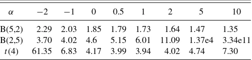
Figure 1represents the cumulative distribution functions and the density functions of two Beta distributions with their cor-responding normal distributions (with equal mean and standard deviation). The parameters of the Beta distributions have been chosen to display divergence from the normal distribution in opposite directions. It is clear fromFigure 1that the Beta(5,2) distribution is skewed to the left and Beta(2,5) is skewed to the right, while the normal distribution is of course unskewed. As can be deduced from (10), in the first case theGαstatistic de-creases asαincreases, whereas in the second case it increases withα.
These observations are confirmed by the results ofTable 1, which shows normality tests withGαbased on single samples of 1000 observations each drawn from the Beta(5,2) and from the Beta(2,5) distributions. Additional results are provided in the table with data generated by Student’s t distribution with four degrees of freedom, denoted t(4). The t distribution is symmetric, and differs from the normal on account of kurtosis rather than skewness. The results inTable 1fort(4) show that Gαdoes not increase or decrease globally withα. However, as this example shows, the sensitivity toαprovides information on the sort of divergence of the data distribution from normality. It is thus important to compare the finite-sample performance of Gαwith that of other standard goodness-of-fit tests.
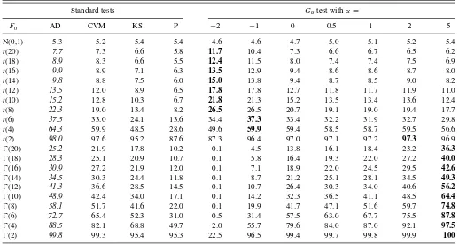
Table 2 presents simulation results on the size and power of normality tests using Student’stand Gamma (Ŵ) distributions
with several degrees of freedom, df =2,4,6, . . . ,20. The t andŴdistributions provide two realistic examples that exhibit different types of departure from normality but tend to be closer to the normal asdf increases. The values given inTable 2are the percentages of rejections of the nullH0:x∼Normal at 5%
nominal level when the true distribution ofx isF0, based on
samples of 100 observations. Rejections are based onbootstrap p-values for all tests, not just those that useGα. WhenF0is the
standard normal distribution (first line), the results measure the Type I error of the tests, by giving the percentage of rejections ofH0 when it is true. For nominal level of 5%, we see that the
Type I error is small. When F0 is not the normal distribution
(other lines of the Table), the results show the power of the tests. The higher a value in the table, the better is the test at detecting departures from normality. As expected, results show that the power of all statistics considered increases asdf decreases and the distribution is further from the normal distribution.
Table 1. Normality tests withGαbased on 1000 observations drawn
from Beta andtdistributions
α −2 −1 0 0.5 1 2 5 10
B(5,2) 2.29 2.03 1.85 1.79 1.73 1.64 1.47 1.35 B(2,5) 3.70 4.02 4.6 5.15 6.01 11.09 1.37e4 3.34e11
t(4) 61.35 6.83 4.17 3.99 3.94 4.02 4.74 7.30
Table 2. Normality tests: Percentage of rejections ofH0:x∼Normal, when the true distribution ofxisF0; sample size = 100, 5000
replications, 999 bootstraps
Standard tests Gαtest withα=
F0 AD CVM KS P −2 −1 0 0.5 1 2 5
N(0,1) 5.3 5.2 5.4 5.4 4.6 4.6 4.7 5.0 5.1 5.2 5.4
t(20) 7.7 7.3 6.6 5.8 11.7 10.4 7.3 6.6 6.7 6.5 6.2
t(18) 8.9 8.3 6.6 5.5 12.4 11.5 8.0 7.4 7.4 7.5 6.9
t(16) 9.9 8.9 7.1 6.3 13.5 12.9 9.4 8.6 8.6 8.7 8.0
t(14) 9.8 8.8 7.5 6.0 15.0 13.8 9.4 8.7 8.5 9.0 8.2
t(12) 13.5 12.0 8.9 6.5 17.8 17.8 12.7 11.8 11.7 11.9 11.0
t(10) 15.2 12.8 10.3 6.7 21.8 21.3 15.2 13.5 13.4 13.6 12.4
t(8) 22.3 19.0 13.4 8.2 26.5 26.5 20.7 19.1 19.0 19.4 17.7
t(6) 37.5 33.0 24.1 13.6 34.4 37.3 33.4 32.2 31.9 32.7 29.8
t(4) 64.3 59.9 48.5 28.6 49.6 59.9 59.4 58.5 58.7 59.5 56.6
t(2) 98.0 97.6 95.2 87.6 87.3 96.4 97.0 97.1 97.2 97.3 96.9
Ŵ(20) 25.2 21.9 17.8 10.2 0.1 4.5 13.8 16.1 18.4 23.2 36.3
Ŵ(18) 28.3 25.1 20.9 10.7 0.1 5.8 16.4 19.3 22.0 27.2 40.0
Ŵ(16) 30.9 27.2 21.9 12.0 0.1 7.1 18.9 22.0 24.5 29.5 42.6
Ŵ(14) 34.5 30.3 24.4 11.8 0.1 8.7 21.2 25.1 28.1 34.5 49.3
Ŵ(12) 41.3 36.6 28.5 14.5 0.1 10.7 26.4 30.3 34.0 40.6 56.2
Ŵ(10) 48.9 42.4 34.0 17.1 0.1 14.2 32.3 36.5 41.1 48.5 64.4
Ŵ(8) 58.1 51.7 41.6 22.0 0.1 19.9 41.7 47.1 51.6 59.7 74.8
Ŵ(6) 72.7 65.4 52.3 31.0 0.5 31.4 57.5 63.0 67.7 75.5 87.8
Ŵ(4) 88.5 82.1 68.8 49.7 2.0 55.7 79.6 84.0 87.0 92.1 97.5
Ŵ(2) 99.8 99.3 95.4 95.3 22.5 96.5 99.4 99.7 99.8 99.9 100
Among the standard goodness-of-fit tests,Table 2shows that the AD statistic is better at detecting most departures from the normal distribution (italic values). The CVM statistic is close, but KS and P have poorer power. Similar results are found in Stephens (1986). Indeed, the Pearson chi-square test is usually not recommended as a goodness-of-fit test, on account of its inferior power properties.
Among theGα goodness-of-fit tests,Table 2shows that the detection of greatest departure from the normal distribution is sensitive to the choice ofα. We can see that, in most cases, the most powerfulGαtest performs better than the most powerful standard test (bold vs. italic values). In addition, it is clear thatGαincreases withαwhen the data are generated from the Gamma distribution. This is because the Gamma distribution is skewed to the right.
4.2 Tests for Other Distributions
Table 3presents simulation results on the power of tests for the lognormal distribution.5 The values given in the table are the percentages of rejections of the nullH0:x ∼lognormal at
level 5% when the true distribution ofxis the Singh–Maddala distribution—see Singh and Maddala (1976)—of which the dis-tribution function is
FSM(x)=1−(1+(x/b)a)−p
5Results under the null are close to the nominal level of 5%. Forn
=50, we obtain rejection rates, for AD, CVM, KS, Pearson, and G with α= −2,−1,0,0.5,1,2,5, respectively, of 5.02, 4.78, 4.76, 4.86, 5.3, 5.06, 4.88, 4.6, 4.72, 5.18.
with parametersb=100, a=2.8, andp=1.7. We can see that the most powerfulGαtest (α=1) performs better than the most powerful standard test (bold vsitalic values). The least powerfulGαtest (α=5) performs similarly to the KS test.
Table 4presents simulation results on the power of tests for the Singh–Maddala distribution. The values given in the table are the percentage of rejections of the nullH0:x∼SM at 5%
when the true distribution ofxis lognormal. We can see that the most powerfulGα test (α=5) performs better than the most powerful standard test (boldvs.italic values).
Note that the two experiments concern the divergence be-tween Singh–Maddala and lognormal distributions, but in op-posite directions. For this reason theGαtests are sensitive toα in opposite directions.
4.3 Application
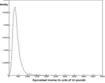
Finally, as a practical example, we take the problem of mod-eling income distribution using the U.K. Households Below Average Incomes 2004–2005 dataset. The application uses the “before housing costs” income concept, deflated and equival-ized using the OECD equivalence scale, for the cohort of ages 21–45, couples with and without children, excluding households with self-employed individuals. The variable used in the dataset is oe bhc. Despite the name of the dataset, it covers the entire in-come distribution. We exclude households with self-employed individuals as reported incomes are known to be misrepresented. The empirical distribution ˆF consists of 3858 observations and has mean and standard deviation (398.28,253.75).Figure 2 shows a kernel-density estimate of the empirical distribution, from which it can be seen that there is a very long right-hand tail, as usual with income distributions.
Figure 2. Density of the empirical distribution of incomes.
Table 3. Lognormality tests: Percentage of rejections ofH0:x∼lognormal, when the true distribution ofxis
Singh–Maddala(100,2.8,1.7); 5000 replications, 499 bootstraps
Standard tests Gαtest withα=
nobs AD CVM KS P −2 −1 0 0.5 1 2 5
50 20.4 18.2 14.5 9.4 32.2 33.7 25.7 21.3 19.3 17.4 12.4 100 33.7 30.2 23.1 11.4 46.0 49.0 37.8 33.3 31.0 28.2 18.1 200 56.2 51.5 40.6 17.4 65.7 70.3 59.3 55.5 53.1 50.1 36.1 300 73.9 69.4 56.9 24.6 81.0 84.3 76.4 73.0 71.0 68.1 55.4 400 84.3 80.2 68.5 31.8 89.0 91.5 85.7 83.5 82.2 79.9 69.2 500 90.6 87.7 77.7 38.7 93.8 95.0 91.5 90.0 89.1 87.5 79.5
Table 4. Singh–Maddala tests: percentage of rejections ofH0:x∼SM, when the true distribution ofxis
lognormal(0,1); 1000 replications, 199 bootstraps
Standard tests Gαtest withα=
nobs AD CVM KS P −2 −1 0 0.5 1 2 5
500 53.6 43.3 32.3 16.7 11.3 37.3 47.7 50.2 53.0 57.4 73.5 600 65.8 52.6 37.4 20.1 18.6 51.3 60.1 62.4 64.5 68.4 83.3 700 75.7 61.8 43.7 22.8 24.9 61.4 71.5 73.3 74.4 77.9 87.4 800 82.3 69.3 53.1 27.6 37.9 72.5 79.3 80.6 82.6 85.8 93.6 900 87.7 75.9 54.8 30.6 45.8 77.5 82.9 83.9 85.6 88.5 93.7 1000 91.2 80.9 62.8 34.2 55.7 82.6 86.9 88.1 89.4 92.4 96.4
Table 5. Standard goodness-of-fit tests: Bootstrapp-values, H0:x∼lognormal
Test AD CVM KS P
Statistic 47.92 1.857 0.034 85.54 p-value 0 0 0 0
We test the goodness of fit of a number of distributions often used as parametric models of income distributions. We can im-mediately dismiss the Pareto distribution, the density of which is a strictly decreasing function for arguments greater than the lower bound of its support. First out of more serious possibili-ties, we consider the lognormal distribution. InTable 5, we give the statistics and bootstrapp-values, with 999 bootstrap samples
Table 6. Gαgoodness-of-fit tests: Bootstrapp-values,
H0:x∼lognormal
α −2 −1 0 0.5 1 2 5
Statistic 1.16e21 9.48e8 7.246 7.090 7.172 7.453 8.732 p-value 0 0 0 0 0 0 0
Table 7. Standard goodness-of-fit tests: Bootstrapp-values, H0:x∼SM
Test AD CVM KS P
Statistic 0.644 0.050 0.010 13.37 p-value 0.028 0.274 0.305 0.050
Table 8. Gαgoodness-of-fit tests: Bootstrapp-values,H0:x∼SM
α −2 −1 0 0.5 1 2 5
Statistic 164.3 1.362 0.441 0.404 0.390 0.382 0.398 p-value 0.002 0 0.006 0.011 0.013 0.014 0.013
Table 9. Standard goodness-of-fit tests: Bootstrapp-values, H0:x∼Dagum
Test AD CVM KS P
Statistic 0.773 0.067 0.011 14.904 p-value 0.009 0.124 0.141 0.027
Table 10. Gαgoodness-of-fit tests: Bootstrapp-values,
H0:x∼Dagum
α −2 −1 0 0.5 1 2 5
Statistic 59.419 1.148 0.576 0.553 0.548 0.556 0.619 p-value 0.001 0 0 0 0 0 0.001
used to compute them, for the standard goodness-of-fit tests, and then, inTable 6, thep-values for theGαtests.
Every test rejects the null hypothesis that the true distribution is lognormal at any reasonable significance level.
Next, we tried the Singh–Maddala distribution, which has been shown to mimic observed income distributions in various countries, as shown by Brachman, Stich, and Trede (1996). Table 7presents the results for the standard goodness-of-fit tests; Table 8results for theGαtests. If we use standard goodness-of-fit statistics, we would not reject the Singh–Maddala distribution in most cases, except for the Anderson–Darling statistic at the 5% level.
Conversely, if we useGαgoodness-of-fit statistics, we would reject the Singh–Maddala distribution in all cases at the 5% level. Our previous simulation study showsGα and AD have better finite sample properties. This leads us to conclude that the Singh–Maddala distribution is not a good fit, contrary to the conclusion from standard goodness-of-fit tests only.
Finally, we tested goodness of fit for the Dagum distribution, for which the distribution function is
FD(x)=
1+
b x
a−p ;
see Dagum (1977) and Dagum (1980). Both this distribution and the Singh–Maddala are special cases of the generalized beta distribution of the second kind, introduced by McDonald (1984). For further discussion, see Kleiber (1996), where it is remarked that the Dagum distribution usually fits real income distributions better than the Singh–Maddala. The results, in Tables 9 and 10, indicate clearly that, at the 5% level of significance, we can reject the null hypothesis that the data were drawn from a Dagum distribution on the basis of the Anderson–Darling test, the Pearson chi-square, and, still more conclusively, for all of
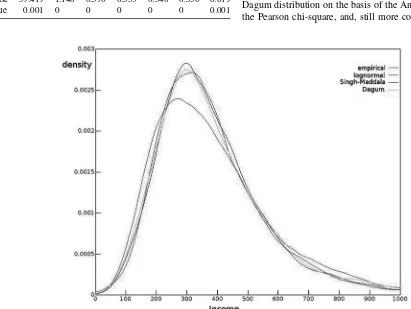
Figure 3. Densities of the empirical and three fitted distributions.
theGαtests. For this dataset, therefore, although we can reject both the Singh–Maddala and the Dagum distributions, the latter fits less well than the former.
For all three of the lognormal, Singh–Maddala, and Dagum distributions, theGα statistics decrease with αexcept for the higer values ofα. This suggests that the empirical distribution is more skewed to the left than any of the distributions fitted to one of the families.Figure 3shows kernel density estimates of the empirical distribution and the best fits from the lognormal, Singh–Maddala, and Dagum families. The range of income is smaller than that in Figure 2, so as to make the differences clearer. The poorer fit of the lognormal is clear, but the other two families provide fits that seem reasonable to the eye. It can just be seen that, in the extreme left-hand tail, the empirical distribution has more mass than the fitted distributions.
5. CONCLUDING REMARKS
The family of goodness-of-fit tests presented in this article has been seen to have excellent size and power properties as compared with other, commonly used, goodness-of-fit tests. It has the further advantage that the profile of theGαstatistic as a function ofαcan provide valuable information about the nature of the departure from the target family of distributions, when that family is wrongly specified.
We have advocated the use of the parametric bootstrap for tests based on Gα. The distributions of the limiting random variables (11) and (A.31) exist, as shown, but cannot be con-veniently used without a simulation experiment that is at least as complicated as that involved in a bootstrapping procedure. In addition, there is no reason to suppose that the asymptotic distributions are as good an approximation to the finite-sample distribution under the null as the bootstrap distribution. We rely on the mere existence of the limiting distribution to justify use of the bootstrap. The same reasoning applies, of course, to the conventional goodness-of-fit tests studied in Section4. They too give more reliable inference in conjunction with the parametric bootstrap.
Of course, theGαstatistics for different values ofαare cor-related, and so it is not immediately obvious how to conduct a simple, powerful, test that works in all cases. It is clearly inter-esting to computeGαfor various values ofα, and so a solution to the problem would be to use as test statistic the maximum value ofGαover some appropriate range ofα. The simulation results in the previous section indicate that a range ofαfrom−2 to 5 should be enough to provide ample power. It would probably be inadvisable to consider values ofαoutside this range, given that it is for α=2 that the finite-sample distribution is best approximated by the limiting asymptotic distribution. However, simulations, not reported here, show that, even in conjunction with an appropriate bootstrap procedure, use of the maximum value leads to greater size distortion than forGαfor any single value ofα.
APPENDIX OF PROOFS
Proof of Theorem 1.Axioms 1–4 imply thatcan be represented by a continuous function:Zn
→Rthat is increasing in|ui−vi|,
i=1, . . . , n. By Axiom 3, part (a) of the result follows from Theorem
5.3 of Fishburn (1970). This theorem says further that the functions φiare unique up to similar positive linear transformations; that is, the
representation of the weak ordering is preserved ifφi(z) is replaced by
ai+bφi(z) for constantsai,i=1, . . . , n, and a constantb >0. We
may, therefore, choose to define theφi such thatφi(0,0)=0 for all
i=1, . . . , n.
Now takez′andzas specified in Axiom 4. From (1), it is clear that z∼z′if and only if
φi(ui+δ, ui+δ)−φi(ui, ui)+φj(uj−δ, uj−δ)
−φj(uj, uj)=0
which can be true only if
φi(ui+δ, ui+δ)−φi(ui, ui)=f(δ)
for arbitraryuiandδ. This is an instance of the first fundamental Pexider
functional equation. Its solution implies thatφi(u, u)=ai+biu. But
above we chose to setφi(0,0)=0, which implies thatai=0, and that
φi(u, u)=biu. This is Equation (2).
Proof of Theorem 2. The function introduced in the proof of Theorem 1 can, by virtue of (1), be chosen as
(z)=
n
i=1
φi(zi). (A.1)
Then the relationz∼z′ implies that (z)=(z′). By Axiom 5, it
follows that, if(z)=(z′), then(tz)=(tz′), which means that
is a homothetic function. Consequently, there exists a functionθ : R→Rthat is increasing in its second argument, such that
n
i=1
φi(t zi)=θ t, n
i=1
φi(zi)
. (A.2)
The additive structure ofimplies further that there exists a function ψ :R→Rsuch that, for eachi=1, . . . , n,
φi(t zi)=ψ(t)φi(zi). (A.3)
To see this, choose arbitrary distinct valuesjandkand setui=vi=0
for alli=j, k. Then, sinceφi(0,0)=0, (A.2) becomes
φj(t uj, t vj)+φk(t uk, t vk)=θ(t, φj(uj, vj)+φk(uk, vk))
(A.4)
for allt >0, and for all (uj, vj),(uk, vk)∈Z. Let us fix values fort,
vj, andvk, and consider (A.4) as a functional equation inuj anduk.
As such, it can be converted to a Pexider equation, as follows. First, let fi(u)=φi(t u, t vi),gi(u)=φi(u, vi) fori=j, k, andh(x)=θ(t, x),
With these definitions, Equation (A.4) becomes
fj(uj)+fk(uk)=h(gj(uj)+gk(uk)). (A.5)
Next, letxi=gi(ui) andγi(x)=fi gi−1(x)
, fori=j, k. This trans-forms (A.5) into
γj(xj)+γk(xk)=h(xj+xk),
which is an instance of the first fundamental Pexider equation, with solution
γi(xi)=a0xi+ai, i=j, k, h(x)=a0x+aj+ak,
(A.6)
where the constantsa0,aj, andakmay depend ont,vj, andvk. In terms
of the functionsfiandgi, (A.6) implies thatfi(ui)=a0gi(ui)+ai, or,
with all possible functional dependencies made explicit,
φj(t uj, t vj)=a0(t, vj, vk)φj(uj, vj)+aj(t, vj, vk) (A.7)
and
φk(t uk, t vk)=a0(t, vj, vk)φk(uk, vk)+ak(t, vj, vk). (A.8)
If we construct an equation like (A.7) forjand another indexl=j, k, we get
φj(t uj, t vj)=d0(t, vj, vl)φj(uj, vj)+dj(t, vj, vl) (A.9)
for functionsd0 anddj that depend on the arguments indicated. But,
since the right-hand sides of (A.7) and (A.9) are equal, that of (A.7) cannot depend onvk, since that of (A.9) does not. Thusajcan depend
at most ontandvj, whilea0, which is the same for bothjandk, can
depend only ont; we writea0=ψ(t). Thus Equations (A.7) and (A.8)
both take the form
φi(t ui, t vi)=ψ(t)φi(ui, vi)+ai(t, vi), (A.10)
where the functionai(vi, t) no longer appears. Then, in view of Acz´el
and Dhombres (1989, p. 346), there must existc∈Rand a function
identically equal to zero leads to a contradiction. For this assumption implies that neitherψ(t)−tnorbican be identically zero. Then, from
(A.12) and the definition ofλi, we would have
φi(ui, vi)=ucihi(vi/ui)+bivi. (A.13)
With (A.13), Equation (A.2) can be satisfied only ifc=1, as other-wise the two terms on the right-hand side of (A.13) are homogeneous with different degrees. But, ifc=1, bothφ(ui, vi) andλi(ui, vi) are
homogeneous of degree 1, which means thatψ(t)=t, in contradiction with our assumption.
It follows thatai(t, vi)=0 identically. Ifψ(t)=t, we havec=1,
and Equation (A.13) becomes
φi(ui, vi)=uihi(vi/ui)+bivi. (A.14)
Ifψ(t) is not identically equal tot,bimust be zero for alli, and (A.13)
becomes
φi(ui, vi)=ucihi(vi/ui). (A.15)
Equations (A.14) and (A.15) imply the result (4).
Proof of Theorem 3.With Axiom 6 we may rule out the case in which thebi=0 in (4), according to which we would haveφi(ui, vi)=
forx >1. Now take the special case in which, in distributionz′
0, the
discrepancy takes the same valuerin allnclasses. If (ui, vi) represents
a typical component inz0, thenz0∼z′
Axiom 6 requires that, in addition,
n
contradicts the assumption that thebiare zero. Consequently, theφiare
given by the representation (A.14), wherec=1. Letgi(x)=hi(x)+
one in thesi, whence the function
n
by an argument exactly like that in the proof of Theorem 2, we conclude that
With our definitions, this means that
uigi(t si)=a0(t)uigi(si)+ai(t, ui). (A.19)
as an identity intandsi. The identity looks a little simpler if we define
ki(x)=gi(x)−bi, which implies thatki(1)=0. Then (A.20) can be
written as
ki(t si)=a0(t)ki(si)+ki(t). (A.21)
The remainder of the proof relies on the following lemma.
Lemma A.1. The general solution of the functional equationk(t s)= a(t)k(s)+k(t) witht >0 ands >0, under the condition that neither anorkis identically zero, isa(t)=tαandk(t)
=c(tα
−1), whereα andcare real constants.
Proof. Let t=s=1. The equation is k(1)=a(1)k(1)+k(1), which implies thatk(1)=0 unlessa(1)=0. But if a(1)=0, then the equation givesk(s)=k(1) for alls >0, which in turn implies that k(1)=k(1)(a(t)+1), which implies thata(t)=0 identically, or that k(1)=k(t)=0. Since we exclude the trivial solutions witha ork identically zero, we must havea(1)=0 andk(1)=0.
Sincek(t s)=k(st), the functional equation implies that
a(t)k(s)+k(t)=a(s)k(t)+k(s), or
for some real constantc. Thusk(t)=c(a(t)−1), and substituting this in the original functional equation and dividing bycgives
a(t s)−1=a(t)(a(s)−1)+a(t)−1=a(t)a(s)−1,
so thata(t s)=a(t)a(s). This is the fourth fundamental Cauchy func-tional equation, of which the general solution isa(t)=tα, for some
realα. It follows immediately thatk(t)=c(tα
−1), as we wished to show.
Proof of Theorem 3 (continued).
The lemma and Equation (A.21) imply that a0(x)=xα and
result of Theorem 3, we may write
(z)=φ¯
where ¯uand ¯vare parameters of the function ¯φthat is the counterpart ofφin (5). It is reasonable to require that(z) should be zero whenz represents a “perfect fit.” A narrow interpretation of zero discrepancy is thatvi=ui,i=1, . . . , n. In this case, we see from (A.23) that
aggregate discrepancy index must be based on individual terms that all use the same value forbi.
This implies that ¯φis homogeneous of degree zero in its three argu-ments. But the value of(z) is also unchanged if we rescale only the vi, multiplying them byk, and so the expression
¯
discrepancy index can be written as
¯
This new functionψ1 is still homogeneous of degree zero in its three
arguments, and so it can be expressed as a function of only two argu-ments, as follows:
The value ofψ2is unchanged if we rescale theviwhile leaving theui
unchanged, and so we have, identically,
ψ2
where we define two functions, each of one scalar argument,ψ4and
ψ.
The discrepancy index in the form (A.25) is therefore given by
ψ In order for the discrepancy index to be zero for a perfect fit with ui=vi, we require thatψ (1/u)¯
n i=1ui
=ψ(1)=0, orφ(n)=0.
Proof of Theorem 5.We make use of a result concerning the em-pirical quantile process; see van der Vaart and Wellner (1996, example 3.9.24). LetFbe a distribution function with continuous positive deriva-tivefdefined on a compact support. Let ˆFnbe the empirical distribution
function of an IID sample drawn fromF, and letQ(p)=F−1(p) and
ˆ
Qn(p)=Fˆn−1(p),p∈[0,1], be the corresponding quantile functions.
Since ˆF is a discrete distribution, ˆQn(p) is just the order statistic
in-dexed by⌈np⌉of the sample. Here⌈x⌉denotes the smallest integer not less thanx. Then
where the notationmeans that the left-hand side, considered as a stochastic process defined on [0,1], converges weakly to the distribu-tion of the right-hand side, wherefis the density of distributionF, and whereB(p) is a standard Brownian bridge as defined in the statement of the theorem.
The U(0,1) distribution certainly has compact support [0,1], and its density is constant and equal to 1 on that interval. The result (A.26) in this case reduces to
√
n u⌈np⌉−p
B(p). (A.27)
We will be chiefly interested in the argumentstidefined asi/(n+1),
i=1, . . . , n. Then we see that √
n(ui−ti)B(ti). (A.28)
This result expresses the asymptotic joint distribution of the uniform order statistics. Note that E(ui)=ti.
Writeui=ti+zi, where E(zi)=0. From (A.27), we see that the
variance ofn1/2z
i isti(1−ti) plus a term that vanishes asn→ ∞6.
Thuszi=Op(n−1/2) asn→ ∞. We express the statisticGα(F,F),ˆ
under the null hypothesis that theuido indeed have the joint distribution
of the uniform order statistics, replacinguibyti+ziand discarding
6In fact, the true variance ofz
iisti(1−ti)/(n+2).
terms that tend to 0 asn→ ∞. We see that
Now, by Taylor’s theorem,
ti
Using Taylor’s theorem once more, we see that
µα
in probability. Putting together Equations (A.31) and (A.32) gives
n
It is striking that the leading-order term in (A.33) does not depend onα. For finiten,Gαdoes of course depend onα. Simulation shows
that, even fornas small as 10, the distributions ofGαand of the leading
term in (A.33) are very close indeed forα=2, but that, forneven as large as 10,000, the distributions are noticeably different for values of αfar enough removed from 2. The reason for this phenomenon is of course the factor ofα−2 in the remainder terms in (A.30) and (A.32). If the limiting asymptotic distribution ofGαexists, it is the same as
that of the approximation in (A.33), and, if the latter exists, it is the distribution of the limiting random variable obtained by replacingzi
byn−1/2B(t
Above, the symbol=d signifies equality in distribution, and the last
step follows on noting that the second last expression is a Riemann sum that approximates the integral.
Similarly, we see that
n
in agreement with (11) in the statement of the theorem.
Proof of Theorem 6.Defineg(v, θ) to bep Q(v, θ), θ. As before,
leading order asymptotically, a calculation exactly like that leading to (A.33) gives
This asymptotic expression depends explicitly onθ, and also on the estimator ˆθthat is used. To show that there does exist a limiting dis-tribution for (A.37), note that, by the definition of the functionh, we have the order statisticsx(i). Then a short Taylor expansion gives
n1/2s(θ)
derivative ofhwith respect to its first argument.
Now, again by use of an argument based on a Riemann sum, we see that
because the expectation ofh(x, θ) is zero. (The integration over the whole real line means in fact integration over the support of the dis-tributionF.) Thus the first term in the sum in (A.39) isO(n−1/2) and
can be ignored for the asymptotic distribution. For the second term, we
replacezias before byn−1/2B(ti) to get
n1/2s(θ)
1
0
h′(Q(t, θ), θ)
f(Q(t, θ), θ)B(t) dt
=
∞
−∞
h′(x, θ)B(F(x, θ)) dx, (A.40)
where for the last step we make the change of variablesx=Q(t, θ), and note that dF(x, θ)=f(x, θ) dx.
Next consider the sum
n−1/2
n
i=1
(zi+g⊤(ti, θ)s(θ))
that appears in (A.37). By the definition ofg,g(ti, θ)=p(Q(ti, θ), θ).
Hence, with error of ordern−1, we have
n−1
n
i=1
g(ti, θ)=n−1 n
i=1
p Q(ti, θ), θ
= 1
0
p Q(t, θ), θdt=
∞
−∞
p(x, θ) dF(x, θ)=P(θ).
Using (A.40), we have
n−1/2
n
i=1
g⊤(t
i, θ)s(θ)P⊤(θ)
∞
−∞
h′(x, θ)B F(x, θ)dx,
and so
n−1/2
n
i=1
zi+g⊤(ti, θ)s(θ)
1
0
B(t) dt+P⊤(θ)
∞
−∞
h′(x, θ)B F(x, θ)dx.
(A.41)
Finally, we consider the first sum in (A.37). By arguments similar to those used above, we see that
n
i=1
zi+g⊤(ti, θ)s(θ)
2
ti
1
0
1 t
B(t)+p⊤ Q(t, θ), θ
×
∞
−∞
h′(x, θ)B F(x, θ)dx2dt.
(A.42)
By combining (A.37), (A.41), and (A.42), we get (14).
[Received July 2012. Revised March 2014.]
REFERENCES
Acz´el, J., and Dhombres, J. G. (1989),Functional Equations in Several Vari-ables, Cambridge: Cambridge University Press. [64]
Anderson, T. W., and Darling, D. A. (1952), “Asymptotic Theory of Certain ‘Goodness-of-Fit’ Criteria Based on Stochastic Processes,”Annals of Math-ematical Statistics, 23, 193–212. [54,58]
Brachman, K., Stich, A., and Trede, M. (1996), “Evaluating Parametric Income Distribution Models,”Allgemeines Statistisches Archiv, 80, 285–298. [62] Dagum, C. (1977), “A New Model of Personal Income Distribution:
Specifica-tion and EstimaSpecifica-tion,”Economie Appliqu´ee, 30, 413–437. [62]
——— (1980), “The Generation and Distribution of Income, the Lorenz Curve and the Gini Ratio,”Economie Appliqu´ee, 33, 327–367. [62]
Davidson, R., and MacKinnon, J. G. (2000), “Bootstrap Tests: How Many Bootstraps,”Econometric Reviews, 19, 55–68. [58]
——— (2006), “Bootstrap Methods in Econometrics,” Chapter 23 ofPalgrave Handbook of Econometrics(Vol. 1), Econometric Theory, eds. T. C. Mills, and K. Patterson, London: Palgrave-Macmillan. [58]
Davison, A. C., and Hinkley, D. V. (1997),Bootstrap Methods and Their Appli-cation, Cambridge: Cambridge University Press. [58]
Ebert, U. (1988), “Measurement of Inequality: An Attempt at Unification and Generalization,”Social Choice and Welfare, 5, 147–169. [54]
Fishburn, P. C. (1970),Utility Theory for Decision Making, New York: Wiley. [63]
Horowitz, J. L. (1997), “Bootstrap Methods in Econometrics: Theory and Nu-merical Performance,” inAdvances in Economics and Econometrics: Theory and Applications(Vol. 3), eds. D. M. Kreps, and K. F. Wallis, Cambridge: Cambridge University Press, pp. 188–222. [58]
Kleiber, C. (1996), “Dagum vs. Singh-Maddala Income Distributions,” Eco-nomics Letters, 53, 265–268. [62]
Kullback, S., and Leibler, R. A. (1951), “On Information and Sufficiency,” Annals of Mathematical Statistics, 22, 79–86. [56]
McDonald, J. B. (1984), “Some Generalized Functions for the Size Distribution of Income,”Econometrica, 52, 647–663. [62]
Moore, D. S. (1986), “Tests of the Chi-Squared Type,” inGoodness-of-Fit Techniques, eds. R. B. D’Agostino, and M. A. Stephens, New York: Marcel Dekker. [58]
Plackett, R. L. (1983), “Karl Pearson and the Chi-Squared Test,”International Statistical Review, 51, 59–72. [54]
Sen, A. K. (1976a), “Real National Income,”Review of Economic Studies, 43, 19–39. [54]
——— (1976b), “Poverty: An Ordinal Approach to Measurement,” Economet-rica, 44, 219–231. [54]
Singh, S. K., and Maddala, G. S. (1976), “A Function for Size Distribution of Incomes,”Econometrica, 44, 963–970. [60]
Stephens, M. A. (1986), “Tests Based on EDF Statistics,” inGoodness-of-Fit Techniques, eds. R. B. D’Agostino, and M. A. Stephens, New York: Marcel Dekker, pp. 97–193. [54,60]
van der Vaart, A. W., and Wellner, J. A. (1996),Weak Convergence and Empir-ical Processes, New York: Springer-Verlag. [57,65]