www.elsevier.nl / locate / econbase
Can waste improve welfare?
a,b ,* c
Alessandra Pelloni , Robert Waldmann a
School of Economic and Social Studies, University of Manchester, Dover Street, M13 9PL, Manchester, UK
b
` `
Facolta di Econima, Universita di Sassari, Via Rolando 1, 7100, Sassari, Italy c
` `
Facolta di Economia, Universita di Chieti, Viale Pindaro 42, 65167, Pescara, Italy Received 1 October 1997; received in revised form 1 June 1998; accepted 1 May 1999
Abstract
In models with a capital spillover, the market outcome is not Pareto efficient since agents ignore the positive externalities caused by investment. One might conclude that taxes on investment or subsidies to consumption will reduce welfare. However, in a model of endogenous growth, either a small tax on capital income, whose proceeds are wasted, increases growth and welfare or a small marginal subsidy to consumption increases growth and welfare. Also if the tax on capital income does not increase growth, a lump sum tax whose proceeds are wasted increases growth and, for a wide range of parameter values, increases welfare. 2000 Elsevier Science S.A. All rights reserved.
Keywords: Growth; Taxes; Spillover; Labour supply; Welfare JEL classification: E62; H31; O41
1. Introduction
Recently, growth models with an endogenous rate of technical change have provided a new framework for studying the effects of taxation. In these models there can be a much larger quantitative influence of policies on welfare than in the neoclassical model because policies have the potential to influence the growth rate in the long run.
*Corresponding author.
E-mail address: [email protected] (A. Pelloni)
A theoretical prediction, shared by a vast majority of these models, is that distortionary taxes are detrimental to growth as they reduce the incentives to produce and invest.
In Romer (1986) the social rate of return on investment exceeds the private return. Under Romer’s assumptions, an investment tax will reduce the growth rate and levels of utility while subsidies will increase them. See also Romer (1989), Barro and Sala-i-Martin (1992, 1995) (Chap. 4). In one sector convex models of growth without externalities, of the kind introduced by Rebelo (1991), the market outcome is Pareto optimal, so there is no reason to subsidize investment but any tax will reduce the welfare of the representative agent.
Many papers study the descriptive and prescriptive aspects of taxation in two sector models of endogenous growth, in which human capital is accumulated along with physical capital, of the kind first introduced by Lucas (1988). In these analyses no externalities or incompleteness of markets are assumed so all taxes will have negative welfare effects. The issue these papers analyze is how to minimize the excess burden of taxation, given an exogenous path of government expenses. Chamley (1985, 1986) and Judd (1985) have shown that in infinitely lived families exogenous growth models with flat-rate taxes on factor incomes the excess burden is minimized if the tax rate on capital income is zero in the long run. Lucas (1990) shows that the Chamley result holds in a two-sector endogenous growth model. Jones and Manuelli (1992), Jones et al. (1997), Milesi-Ferretti and Roubini (1998a,b) show that the tax rates on capital, labour (human capital) income and on consumption should all be zero in the long run.
However, the effects of taxation on growth have proven difficult to isolate empirically. There is an impressive negative relation between the rate of growth and the ratio of tax revenues to GDP as pointed out by Plosser (1993) for OECD countries. However, this ratio rises with per capita income (Wagner’s Law), in both the cross-section and the time series data sets. Easterly and Rebelo (1993) show that when in a growth regression the level of initial income is included to capture the convergence effect discussed in Barro and Sala-i-Martin (1992), the
1
coefficients of tax variables become insignificant.
In light of this evidence, in this paper we ask whether it is theoretically possible for taxes to have a positive effect on growth and welfare, even when the proceeds are thrown away or rebated lump sum, i.e. even when one abstracts from the possible productive uses of government spending.
The answer turns out to be yes as we show using a one sector model of endogenous growth with an infinitely lived representative agent, where, following Romer (1986), there is a spillover to capital so the social production function is in
1
fact linear in capital. The basic difference in assumptions with respect to this benchmark model is that the decision to supply labour is explicitly analysed. The basic intuition is simply that in our model, both capital taxes and lump sum taxes have an impact on the allocation of resources, because they influence labour supply and, therefore, the rate of return on capital and the rate of growth. In particular, either capital taxes or lump sum taxes can increase growth, by making people work more, even if the tax revenue is thrown away. Moreover we show that this can increase the representative consumer’s welfare. We also show that when a tax on capital income does not increase growth and welfare in balanced growth equilibrium, then growth and welfare will be increased by a consumption subsidy financed by a lump-sum tax
Some examples of economic models in which taxes and / or wasteful spending can increase growth and welfare can be found in the literature; however, these positive effects are generated under assumptions different from ours and highlight, therefore, different aspects of the way in which fiscal policy can affect the economy.
The most famous explanation of how wasteful government spending can increase welfare is that it reduces unemployment via a Keynesian effect on aggregate demand. This is in general predicated assuming some form of nominal or real rigidity in prices or wages. We assume perfect competition and price flexibility, so markets clear and there is no possibility of an aggregate demand shortfall.
Another way in which taxes can be good is when they finance productive government spending, as in Barro (1990), Barro and Sala-i-Martin (1992, 1995), Jones and Manuelli (1992), Turnovsky (1996) and Corsetti and Roubini (1996). Jones and Manuelli (1992) and Uhlig and Yanagawa (1996) show that in an overlapping generation framework taxation of capital can increase growth when its proceeds are used to decrease taxes on labour income as workers are the savers. In models with income inequality, capital taxation can increase welfare by
redistri-2
buting from the rich to the poor. If ex ante identical agents become unequal due to uninsured risk, then redistribution can Pareto improve as pointed out by Aiyagari (1995a) and Braun and Uhlig (1996).
These arguments are not related to ours as we assume a representative agent. Our results are examples of second-best theory. The idea that taxes whose revenue is not used productively must reduce welfare is based on the first-best intuition that a waste of resources has a positive social cost. However, the withdrawal of resources from productive use may have a negative social cost in an
2
economy in which there is an externality to capital accumulation, i.e. in a
3
second-best environment.
In our model, the effects of tax policies depend on whether the market
4
equilibrium of the model is locally indeterminate. Such multiple equilibria make it difficult to study the effect of taxes because outcomes are indeterminate with or without taxes. In such cases, in most of our analysis, we simply assume that, with or without taxes, the economy is always on its balanced growth path. We find that similar results hold under the alternative assumption that, if the market equilibrium is indeterminate, labour supply at time zero is equal to the no-tax balanced growth labour supply even if a tax is introduced. If the market equilibrium is indetermi-nate, capital taxes increase the rate of balanced growth and lump sum taxes and consumption subsidies reduce the rate of balanced growth. If the equilibrium is unique, capital taxes reduce growth and lump sum taxes and consumption subsidies increase growth. Thus, in our model, it is always possible to improve welfare using either a tax on capital income or a consumption subsidy, and for specifications of tastes and technology which are considered plausible by many economists it is possible to achieve the same using a lump sum tax.
While we do not address the issue of optimal taxation directly and focus only on the case in which the government tax rates are constant over time and the government runs a continuously balanced budget, we show that an optimal taxation scheme will not always feature zero rates in the long run, contrary to the conclusions reached in some of the papers considered above. The counter-intuitive effects of lump sum taxation have not, to our knowledge, being noted in the literature on public finance and growth before. In fact, in many analyses, proceeds from taxation are assumed to be rebated lump sum on the assumption that this will not affect growth.
The paper is organized as follows: the model is spelled out in Section 2, where we give a general condition for tastes and technology that implies indeterminacy. A numerical example of indeterminacy is presented in Appendix A. In Section 3 we consider public policy, in particular we note that, if the market outcome is indeterminate, growth and welfare in the balanced growth equilibrium are improved by a capital income tax policy with proceeds returned lump sum (Section 3.1), the same result holds if proceeds are used to fund wasteful government spending (Section 3.2). In contrast, if the market outcome is determinate growth is increased by a lump sum tax with proceeds thrown away
3
In a completely different trade theory context a similar counterintuitive effect is derived by Bhagwati (1980) who shows that the cost of a distortion (in his case a tariff) levied with the aid of resource-using lobbying can be lower than the cost of the same distortion in the absence of lobbying.
4
Recently, there has been a renewed interest in indeterminacy, or alternatively said in the existence of a continuum of equilibria in dynamic economic models, which means that ‘sunspots’ and ‘animal spirits’ can matter. See, among others, Benhabib and Farmer (1996, 1994), Benhabib and Perli (1994),
´
Benhabib and Rustichini (1994), Boldrin and Rustichini (1994), Caballe and Santos (1993), Farmer `
(Section 3.3) and growth and welfare are increased by a consumption subsidy financed through a lump sum tax (Section 3.4). Section 4 draws conclusions.
2. The model
We adopt the basic Romer (1986) model of endogenous growth augmented by allowing for variable labour supply. The economy is formed of identical optimizing households, of identical perfectly competitive firms, and a government. In this section we present a general version of the model including all the taxes and subsidies we consider in this paper. In the following section each specific policy mentioned in the introduction is studied separately, putting all other taxes (or subsidies) to zero to clarify which effect each policy has. The features of the model are described in detail below.
Households: There is a continuum of length one of worker / consumers who
maximize the same CES intertemporal utility function, multiplicatively separable in consumption of the homogeneous good C and the amount of labour they supply,
L[[0,1]:
`
12s
C
2rt
]]
V5
E
e h(L ) dt (1)12s
0
5 2
where s is positive and different from one, r is positive, h(L ) is C and the following two conditions must hold for utility to be increasing in consumption and decreasing in labour:
h(L ).0 (2)
(12s)h9(L ),0 (3)
while the following two conditions must hold for concavity:
(12s)h0(L ),0 (4)
s 2
]]]h0(L )h(L ).(h9(L )) (5)
(s 21)
Eq. (6) gives the instantaneous budget constraint consumers face:
] ] ]
l l
I5r(12t 2 tk k)K1WL2(12t )Cc 2t Ka 2t Cc 1tkrK (6)
5
where I is investment. Households derive their income by renting the capital stock
K (of which all have the same initial endowment) and by supplying labour L to
firms, taking the interest rate r and the wage W as given. Capital income is taxed at
l
a ratet 1 tk k. Consumption is subsidized at a rate t . There are lump sum taxes] c ]
proportional to average capital, t K and to average consumption t C. Finally therea c
]
l
is a lump sum subsidy proportional to average capital incometkrK. Agents, being
atomistic, take these averages as variables beyond their control. In this sense these are lump sum taxes. Since we assume no depreciation, the capital stock evolves according to:
~
K5I (7)
The necessary and sufficient conditions for maximizing utility are that Eq. (6) is respected and:
2s
C h(L )5(12t )c l (8)
12s
h9(L )C
]]] 5 lW (9)
(s 21)
~
l l
] 5 r 2l (12t 2 tk k)r (10)
2rt
lim Kle 50 (11)
t→`
wherel is the multiplier associated with the constraint (6). From (8) and (9) we get:
Ch9(L ) W
]]]]5]]] (12)
(s 21)h(L ) (12t )c
which says that the marginal rate of substitution between leisure and consumption
~
must be equal to their relative price. If we calculate l/l by taking the time derivative of the log of both sides of (8) and substitute the resulting expression for
~
l/l in (10), the Euler equation, rearranging we get the optimal rate of growth of consumption:
l
~ ~ (12t 2 t)r2r
C h9(L )L k k
]5]]1]]]]] (13)
C sh(L ) s
this shows that, for a given labour supply and interest rate, a higher tax rate on capital income leads to a reduced rate of increase in C.
Firms: There is a continuum—for notational convenience again assumed of
length one—of competitive firms. As is standard from Romer (1986) we assume that the production set at the firm level is convex in labour L and capital K and in particular that the individual production function is homogeneous of degree one in
]
individual agent (family or firm) acts in isolation taking the actions of other agents as given but in fact in equilibrium every agent takes the same actions. So average variables are equal to individual variables and, given our normalization of agents,
6
to aggregate variables. Production Y is then assumed to be linear in capital
]
Y5F(LK, K )5KF(L, 1);Kf(L ) (14)
2
where f is C , strictly increasing and strictly concave. Competition among profit maximizing firms and the homogeneity assumption ensure that both factors are paid their marginal products and that these payments exhaust the product, that is
Y5rK1WL (15)
W5Kf9(L ) (16)
r5f(L )2f9(L )L;r(L ) (17)
Government: We have seen that government consumption G does not enter the
utility function of consumers or the production function of firms. That is we want to study the effect of taxes, without considering the possible productive uses of the tax revenue. In this sense G is waste. Notice this is a standard assumption in macromodels. We rule out a market for government bonds and assume that the government runs a balanced budget. Given our normalization of agents the flow government budget constraint can be written
] ]
l l
G1t Cc 1tkrK5(t 1 tk k)rK1ta1t Cc (18) where on the left-hand side we have outflows and on the right-hand side we have inflows. Since average and aggregate variables are the same this simplifies to
G5(tkr1t )Ka (19)
Market equilibrium: In a competitive equilibrium individual and aggregate
variables are the same and prices and quantities are consistent with the (private) efficiency conditions for the households (6), (11), (12) and (13), with factor markets clearing conditions (16) and (17), with the government budget constraint (19) and with goods market clearing, i.e. with the economy wide resource constraint
6
Y5C1I1G (20) Given the equality of individual, average and aggregate variables, and given (15) [which is implied by (16) and (17)], (20) can be obtained by aggregating over the individuals’ and the government budget constraints.
Balanced growth equilibrium: Our analysis of the effects of taxes is mostly
carried out assuming the economy follows a balanced growth path (hence BGP), so we will describe it in some detail.
~
Along a BGP labour supply is a constant, i.e. L50, so we consider the optimal
~
rate of growth of consumption when L50, that is, given (13):
l
r(L )(12t 2 tk k)2r
]]]]]] (21)
s
If we substitute (16) in (12) we obtain:
C (s 21)h(L )
]5f9(L )]]]] (22)
K h9(L )(12t )c
This gives us the optimal ratio between consumption and capital in terms of labour and also shows that along a BGP, C and K will grow at the same rate (hence g) or
l
~ r(12t 2 t)2r ~
C k k K
]5]]]]];g5] (23)
C s K
~
Substituting (7), (16), (17) and (22) in (6) the rate of capital accumulation K /K can also be expressed as a function of L:
~
K h(L )
]K5f(L )2(s 21)]]]](12t )h9(L ) f9(L )2t 2 ta kr(L ) (24)
c
Given (23), an implicit expression for BGP labour supply is given by equating the
~ ~
expression in (21), which is equal to C /C along a BGP, and K /K given by (24):
l
r(L )(12t 2 tk k)2r h(L )
]]]]]]s 5f(L )2(s 21)]]]](12t )h9(L ) f9(L )2t 2 ta kr(L )
c
(25)
Each solution of (25) between 0 and 1 and satisfying the transversality condition
ˆ
(hence TC) will define a BGP level of labour supply (hence L ). Along a BGP, the TC (11), using (8) to substitute for l, becomes
2s 2sgt 2rt
C0 e h e
gt
]]]]]
lim K e0 50
t→` (12t )c
0. 2r 1g(12s)
ˆ
h(L ) l
ˆ ]]]] ˆ ˆ
5f(L )2(s 21) ˆ f9(L )2t 2a (12tk)r(L ) (26)
(12t )hc 9(L )
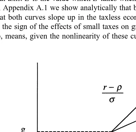
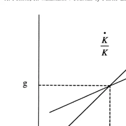
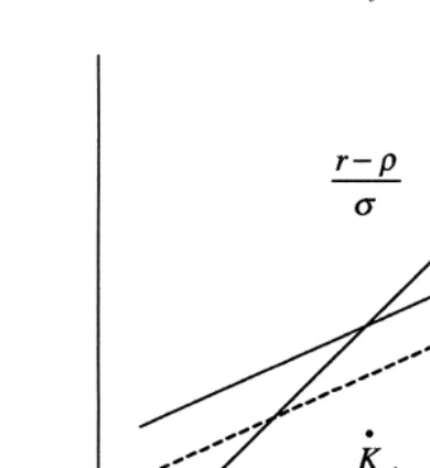
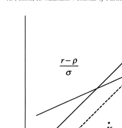
where the equality is obtained by substituting inr 2g(12s) forrits value given by (25) and for g its value given by (24). Since in our policy analysis we assume the economy is in balanced growth, (25) is our key equation for understanding the effects of policies on labour supply and growth. In Section 3 we will use (25) for a series of comparative statics exercises each focused on a specific kind of policy, i.e. we will compare the steady-state equilibrium before and after the introduction of marginal taxes (positive or negative, i.e. transfers) in the taxless economy, which is, therefore, our benchmark economy and to which we turn our attention now. In Figs. 1 and 2 (linearised) sketches of the left-hand side of (25) (giving
~ ~
C /C if L50, which is true along a BGP) and of the right-hand side of (25) (the
~
K /K curve) in the taxless economy are drawn. The intersection of the two curves ˜
gives us g on the vertical axis and the no-tax BGP labour supply L on the
˜ ˆ
[image:9.612.128.348.365.579.2]horizontal axis. L is the value which L takes when T50, where T is the vector of taxes. In Appendix A.1 we show analytically that both curves slope up. We use the result that both curves slope up in the taxless economy repeatedly in Section 3 to evaluate the sign of the effects of small taxes on growth. The fact that both curves slope up, means, given the nonlinearity of these curves, that there can be multiple
Fig. 2. An unstable economy.
solutions, i.e. multiple BGP equilibria. However, we do not analyse the issue in this paper and assume instead that the balanced growth path is unique or, at least, that when a tax is changed marginally the economy does not jump to a new
ˆ
balanced growth path. Formally, we assume that BGP labour supply L is a continuous function of tax rates.
Without taxes, the TC (26) becomes using (17):
˜ h(L )
˜ ]]
L,(s 21) (27)
˜ h9(L )
we notice that since as shown by (26), the expression giving the TC with taxes is
ˆ ˆ
continuous in L and the taxes, for small values of the taxes, and we assume L changes continuously with the taxes, if (27) holds than the transversality condition will hold after the introduction of each small tax.
To ease the presentation we now introduce a new function, N(L ). N(L ) is
~
defined as the difference between the (r(L )2r) /s curve and the K /K curve in the economy with no taxes:
r(L )2r h(L )
]]] ]]
N(L ); s 2f(L )1(s 21) f9(L ) (28)
h9(L )
˜
Since we have defined L as the BGP labour supply in the taxless economy we will
˜
convenient to use (28) to rewrite the BGP equilibrium condition (25) such that consumption and capital grow at the same rate as:
l l
~
r(L )(12t 2 tk k)2r K r(t 1 tk k) tc(12s) h
]]]]]]2]5N(L )2]]]2]]] ] f9 1ta s K s (12tc) h9
1tkr50 (29)
˜
Notice N9(L ) is the difference in slope between the (r(L )2r) /s curve and the
~
K /K curve at their intersection point, in the economy without taxes. This means
˜ ~
that if N9(L ).0 the (r(L )2r) /s curve cuts the K /K curve from below as in Fig.
˜ ~
1, if N9(L ).0 the (r(L )2r) /s curve cuts the K /K curve from below as in Fig. 2.
˜
The sign of N9(L ) is a key determinant both of the effects of marginal taxes as we will see in Section 3 and of the transitional dynamics of the model. Thus, even if our policy results are obtained on the assumption that the economy is always in BGP, there is a link between them and the transitional dynamics in the taxless model which is, therefore, considered below.
Transitional dynamics with no taxes: The equilibrium conditions in the
economy can be reduced to a differential system in K and L. The system is formed by Eq. (24) and by Eq. (30)
N(L ) N(L )
~ ]]]]]]]]]]] ]]
L5 ; (30)
h0(L ) (s 21) h9(L ) f0(L ) D(L )
]] ]]] ]] ]]
2 1 1
S
h9(L ) s h(L ) f9(L )D
~
The algebraic steps to obtain Eq. (30) are given in Appendix A.2. Since L depend on L only, not on K, the stability properties of the BGP equilibrium can be
7
understood focusing on just Eq. (30). To study the dynamic nature of a fixed point
˜ ~ ˜
of Eq. (30), i.e. of BGP labour supply L, we have to sign dL / dL(L ) the derivative
˜ ˜
~ ~
of L with respect to L, calculated at the fixed point L5 L. If dL / dL(L ).0, the
˜
fixed point L is a repeller and the BGP is locally determinate in the sense that if L
˜ ˜
were close to but not exactly equal to L, then L would diverge further from L.
˜
Thus, the BGP with L5L a repeller is a (locally) unique equilibrium path and we
˜ ˜
~
can say that there is no (local) indeterminacy in this case. If dL / dL(L ),0, L is an
˜
attractor, that is if L is near L it will eventually approach it. So there is local indeterminacy i.e. a continuum of equilibrium trajectories all converging to the given BGP. We have:
7
Proposition 1. A balanced growth path in the taxless economy is locally
˜ ˜
indeterminate if N9(L ).0 and locally determinate if N9(L ),0. Proof.
˜ ˜ ˜
~
dL ˜ N9(L ) N(L ) ˜ N9(L )
](L )5]]2]]2D9(L )5]]
dL D(L )˜ D(L )˜ D(L )˜
˜
since N(L )50. D(L ) in Eq. (30) is negative for all L. In fact
h0 (s 21) h9
] ]]] ] 2 1
h9 s h
is negative as an immediate consequence of the condition (5) for the negative definiteness of the Hessian of instantaneous utility, while f0 is negative. But then
˜ ˜
~
dL / dL(L ) signs as 2N9(L ). h
In Appendix A.3 we prove that indeterminacy cannot apply fors .1 and give a
8
parametric example to show that indeterminacy can apply for s ,1.
~
Recalling N(L ) is the difference between the (r(L )2r) /s curve (giving C /C for
~ ~
L50, which is true along a BGP), and the K /K curve and that the two curves
˜ ˜
intersect at BGP labour supply L, the condition for indeterminacy N9(L ).0 has
˜
the following geometric representation: it just means that at L the (r(L )2r) /s ~
curve slopes up more steeply than the K /K curve. This implies that in Fig. 1 an economy with an indeterminate BGP is represented, i.e. an economy in which the fixed point is an attractor, while in Fig. 2 an economy with a determinate BGP is represented, i.e. an economy in which the fixed point is a repeller. Since both curves slope up one can infer that if there are more than one fixed points, at least one of them must be an attractor. In fact given the monotonicity and continuity of the two curves, it is impossible for them to cross twice with one of the curves being flatter than the other at both intersections. To understand the condition on the slope of the two curves first note that in the indeterminate case leisure must be a normal good. Leisure is a normal good if s ,1, which is required for
9
indeterminacy. For local indeterminacy it is sufficient that, if the initial consump-tion to capital ratio is slightly higher than the balanced growth consumpconsump-tion to capital ratio, then the rate of growth of consumption is lower than the rate of
8
For an existence result on indeterminate equilibria in this model see also Pelloni and Waldmann (1998).
9
Differentiating Eq. (12) we get:
d(C /K ) (s 21) h hh0 ]]dL 5]](12t )
S S
]h9 f0 1 12]2D D
f9(h9) c
growth of capital, so the consumption to capital ratio (and, therefore, L ) return to their steady-state values. If leisure is a normal good a high consumption to capital
~
ratio corresponds to low labour supply. If the K /K curve cuts the (r(L )2r) /s
curve from above then the rate of growth of consumption is more sensitive to changes in labour supply than the rate of growth of capital so this low labour supply has a greater effect on the rate of growth of consumption than on the rate of growth of capital and causes the consumption to capital ratio to return to the balanced growth consumption to capital ratio.
In leading one sector growth models a condition for indeterminacy is that labour supply and / or labour demand have non-conventional slopes. For example for indeterminacy to apply in Benhabib and Farmer (1994) and in Farmer and Guo (1994, 1995), who assume utility logarithmic over consumption and a Cobb-Douglas technology labour demand must slope up more steeply than labour supply (or alternatively slope down less steeply than labour supply or finally labour demand must slope up and labour supply must slope down). This is difficult to reconcile with empirical evidence as Aiyagari (1995b) points out. In our model, in contrast, where the intertemporal elasticity of substitution of consumption and the elasticity of substitution between factors can be different from one, both labour demand given capital and labour supply given consumption will have the
10
conventional slopes in the indeterminate case.
3. Some policy experiments
In this section, we study the effect of some combinations of the taxes and subsidies described in the previous section, when introduced in the economy without taxes. Many counter-intuitive effects of policy can be shown. First policies of taxing capital income or of taxing lump sum and throwing away the revenue can be growth and welfare increasing. Moreover even if investment is inefficiently low, a consumption subsidy can cause an increase in the rate of growth and welfare. The same effect would occur if the government forced a higher consumption to capital ratio by decree by, for example, threatening to punish consumers who consume too little. In most of the analysis we assume that the
11
economy with or without taxes is always in balanced growth. As mentioned in the previous section, we assume that the balanced growth path is unique or that if
10
We have from Eq. (12)
2 d(W/C ) 1 h0 (h9)
]]dL 5]]]](12t)(s 21)
S
]h 2]2D
, h cwhich is implied to be positive by Eq. (5), fors ,1. 11
it is not unique the introduction of a tax does not cause the economy to jump to a new balanced growth path. In other words we assume that BGP labour supply is a continuous function of the tax rates. The analysis of transitional dynamics in the previous section is used to show that the signs of the effects of tax policies on the balanced growth equilibrium depend on whether the no-tax balanced growth
˜
labour supply L is an attractor (so that the BGP equilibrium is indeterminate) or a repeller (so that the BGP equilibrium is determinate). In particular, in the first case, taxing capital income and destroying the proceeds is always welfare improving, while in the second case subsidizing consumption is always welfare improving. In all our tax experiments the tax rates are constant though time. Clearly, if it can be shown as we do that, starting from a no-tax situation, the introduction of a permanent tax can improve welfare it is clear that any plan featuring zero tax rates in the steady state cannot be optimal, and in this sense our restricted analysis can
12
be directly compared to those conducted allowing for variable tax rates.
Our investigation involves two types of policy analysis. First we analyse the effect of the policies on growth. This analysis is based on comparative statics analysis of Eq. (25), i.e. done by calculating the total derivative of BGP labour supply with respect to each tax, setting other taxes to zero. Effects of taxes on labour and growth are geometrically illustrated in Figs. 3–7. Second we analyse the effect of the policies on welfare. We consider only small taxes so we focus on their first-order welfare effects. Our technique for evaluating these effects hinges on calculating an expression for maximum welfare V along a BGP in terms of
ˆ
initial K (hence K ), optimal L (i.e. L ) and the taxes. We are then able to sign the0
derivative of V with respect to each marginal tax, setting other taxes to zero, by looking at the conditions for the convexity of technology and preferences and at the TC. We give here those steps for the analysis of welfare effects which are the same for all taxes. From now on in order to simplify the notation we suppress the argument of h, f, of their derivatives and of r—whenever it is not specifically needed. Assuming the economy is always in steady state, the indirect utility function V is
` 12s
C0 h s2r 1g( 12s) td
]]
V5
E
e dt12s
0
22s 12s 12s
12s h K (s 21)
(31)
0
C0 ]]]
S
]]] f9D
]]h (12s) (12t )h9
12s c
]]]]] ]]]]]]]]]]]]]
5 5
h
(r 2g(12s)) l
]]]
(s 21) f9 2f1r(12t )1t
S
(12t )h9 k aD
c
12
The first equality is obtained just by integrating. The second equality is obtained using (26) to substitute forr 2g(12s) and (22) to substitute for C . In general,0
for a taxt(wheretindicates any component of vector T ) to be beneficial, starting from a no-tax equilibrium, we need the total derivative
dV
]
*
.0. dt T50log((12s)V )
]]]]
(12s)
is an increasing transformation of V so its total derivative
ˆ
d(log((12s)V )) ≠(log(12s)V ) dL ≠(log((12s)V ))
]]]]]
*
5]]]]]*
1] ]]]]]*
dt ˆ
(12s) dt T50 (12s)≠t T50 (12s)≠L T50
(32)
signs as
dV
]
*
dt T50
ˆ
and is more tractable, so we will use it. Notice L is used to underline we are considering changes in BGP labour supply. For brevity we suppress the notation
uT50 below, but all derivatives are still to be evaluated at the no-tax BGP
˜
equilibrium, i.e. for T50, L5L. In Appendix A.4 we calculate
≠(log((12s)V ))
]]]]]
(12s)≠L
and show that it is positive if s ,1 and negative if s .1. In the following subsections all is left to be done is to calculate the other derivatives in (32) for each policy.
3.1. Tax on capital, proceeds returned lump sum
We first consider the introduction of a capital income tax, whose proceeds are returned in equal proportions to all consumers. In other words we study the
l
l
r(12tk)2r h
]]]]5f2(s 21)] f9 (33)
s h9
and its equivalent (29)
l
rtk
ˆ ]
N(L )2 s 50 (34)
(34) is easier to differentiate than (33). We have:
˜
Proposition 2. If the no-tax balanced growth L is an attractor, a small tax on
capital whose proceeds are returned as a lump sum increases the rate of growth in the balanced growth equilibrium.
Proof. Differentiating (34) around the BGP equilibrium values without taxes, i.e.
˜
around L5L, T50, we find the following effect on BGP labour supply:
˜ ˆ
dL r(L )
]l 5]]]˜ (35)
dtk sN9(L )
˜ ˜
This is positive if N9(L ).0, that is, if L is an attractor. To prove the effects on g
~
we just have to recall that the right-hand side of (33)—the K /K curve—which is equal to g along a BGP, is increasing in labour, as proved in Appendix A.1. So the effects on growth will be positive if labour increases. h
Our comparative analysis of the BGP equilibrium with and without the tax is
~
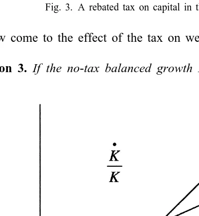
illustrated by Figs. 3 and 4. If starting with no taxes this tax is introduced the K /K curve stays the same while the other curve, giving the optimal rate of consumption
l
~
for L50, moves down from (r2r) /s to (r(12tk)2r) /s. So if the (r2r) /s ~
curve is steeper than the K /K curve the intersection point of two curves after the introduction of the small tax will be on the north east of the previous intersection point, that is the tax and transfer policy will increase labour supply and growth. The following is a heuristic explanation of this somewhat surprising result. In
~
our model, for an unchanged K /K curve higher labour supply implies a higher
˜
Fig. 3. A rebated tax on capital in the stable economy.
We now come to the effect of the tax on welfare.
˜
Proposition 3. If the no-tax balanced growth L is an attractor, a small tax on
[image:17.612.136.336.359.576.2]capital whose proceeds are returned as a lump sum increases welfare in the balanced growth equilibrium.
Proof. We have to calculate the derivatives in (32) for the particular case at hand. From (31) whent 5k 0,t 5c 0,t 5a 0 we derive:
≠(log((12s)V )) r
]]]]]l 5]]]]]]]]h (36)
(12s)≠tk (12s) (
S
s 21)]2L˜D
f9h9
To sign (36) recall the TC (27). We then have (36) is positive if s ,1. It is proved in Appendix A.4 that, if s ,1,
≠(log((12s)V ))
]]]]] .0 (12s)≠L
˜
But this means that all the derivatives in (32) are positive, if L is an attractor (only possible if s ,1), so the tax increases welfare. h
This effect of the policy on welfare can be understood intuitively as follows. If
~
the BGP labour supply increases, the economy moves up the K /K curve, that is investment increases, so the beneficial spillover increases and welfare increases to first order in the change in labour supply. In our model increasing labour supply
˜
slightly above L is welfare increasing as the positive indirect effect through the increase in the interest rate and the externality is stronger than the negative effect due to the increased disutility of labour. Thus, a small tax causes increased welfare.
The small tax and transfer policy also increases welfare if, with the tax, labour
˜
supply at time zero (hence L ) is equal to L, that is assuming that L is equal with0 0
and without the tax so that with the tax the economy is in a non-balanced growth
~
equilibrium. Again the argument is very simple: the tax increases L for any L near the no-tax balanced growth labour supply. Therefore, it causes labour supply to be higher at each t. This means it causes higher investment at each t, and a higher beneficial externality. So even given fixed initial L, the tax causes a first order increase in welfare. A formal proof corresponding to this argument is available to the reader on request.
Even if the balanced growth path is locally indeterminate, it is possible to demonstrate an effect of taxes on long run growth without making assumptions about which equilibria are selected with and without taxes. The asymptotic growth rate without taxes is lower than the asymptotic growth rate with a small tax on
˜
equilibrium with taxes and any equilibrium without taxes, output and growth will
13
eventually become and remain higher with the tax policy than without.
3.2. Tax on capital, proceeds thrown away
We will now analyse the steady-state effects on growth and welfare of a tax on capital incometk, whose proceeds are used to pay for expenditures G 5rtk that enter neither households’ utility functions nor firms’ production functions. In other
l
words we study the particular case in whicht 5k 0,t .k 0,t 5c 0,t 5a 0. Again, as in all our tax experiments we assume that, with or without a tax, the economy is in balanced growth. The BGP equality between the rates of growth of consumption and capital (25) becomes:
(12tk)r2r h
]]]]s 5f2(s 21)]h9 f9 2rtk (37) We then have:
˜
Proposition 4. If the no-tax balanced growth L is an attractor, a small wasted tax
on capital increases the rate of growth and welfare in the balanced growth equilibrium.
Proof. From (29), which is a way to rewrite (25), we see that (37) can be written as
tk(12s)r
ˆ ]]]
N(L )2 50,
s
˜
that is, differentiating (37) around the no-tax equilibrium L5L, T50 we find
˜ ˆ
dL (12s)r(L )
]5]]]] (38)
dtk sN9(L )˜
˜ ˜
We recall that N9(L ).0 is the condition for indeterminacy. So if L is an attractor (which is only possible fors ,1) the tax will always increase labour supply. The partial derivative of V with respect totk, when V is expressed as in (31), is zero as
tk does not appear in the expression. Thus, to calculate whether introducing the tax can be beneficial, we just have to consider
13
If there are multiple balanced growth equilibria we can say the following: If the balanced growth ˜
ˆ
≠V dL
] ].
ˆ dt ≠L k
ˆ
In Appendix A.4 we prove that ≠V/≠L is positive if s ,1. Therefore, the tax on capital increases BGP welfare if s is less than one and the tax causes increased
˜ ˜
labour supply. Both conditions are respected if L is an attractor. Notice that if L is an attractor the tax will increase g as well. In fact whens is less than one, leisure and the ratio between consumption and capital must move together. So the tax will reduce consumption at time 0 and leisure at all times. But since V is an increasing
ˆ
function of C /K , 10 0 2L and g, given K , the result that the tax increases welfare0
implies that it increases g. h
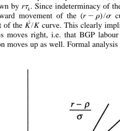
In Fig. 5 the left-hand side and the right-hand side of (37) are represented, with and without the tax, in the case of an indeterminate BGP equilibrium in the taxless
~
economy, i.e. in the case in which the (r2r) /s curve is steeper than the K /K curve in the neighborhood of the equilibrium. When the tax is introduced the
~
(r2r) /s curve is replaced by the lower (r(12tk)2r) /s, while the K /K curve moves down by rtk. Since indeterminacy of the BGP impliess ,1, we have that the downward movement of the (r2r) /s curve is bigger than the downward
~
movement of the K /K curve. This clearly implies that the intersection between the two curves moves right, i.e. that BGP labour supply increases. In the figure the
ˆ
[image:20.612.140.337.361.576.2]intersection moves up as well. Formal analysis shows that if L increases ands ,1
ˆ
the increase in L outweighs the negative direct effect (for fixed L ) of the tax on g
14
and the interest rate, so that g always increases.
The result can be intuitively explained by noticing that here a mechanism is at work similar to that delivering the result that a rebated tax on capital can increase labour supply and growth. Suppose we start from a market equilibrium and we move to another equilibrium with a higher labour supply (and a lower initial consumption). As seen in the previous section such new equilibrium cannot be a
˜
BGP equilibrium if L is an attractor because at the higher labour supply the rate of growth of consumption will be higher than the rate of growth of capital, causing labour supply eventually to decline all the way back to the old equilibrium. To make the higher labour supply sustainable in the long run the rate of growth of consumption will have to decrease more than the rate of growth of capital, for each level of labour. A tax on capital income has this effect, whether its proceeds are rebated or thrown away. However, in the latter case the tax is a less powerful instrument to increase the BGP labour supply than in the former case. In fact if the proceeds are thrown away instead of being rebated, the tax will reduce not only the rate of growth of consumption but also the rate of growth of capital. However, what determines the sign of the effect on labour supply is that the impact of the tax on the former is stronger than the impact on the latter. We have seen that this is true ifs ,1, as then the effect of the tax on the rate of growth of consumption,
~
measured by rtk/s, is higher than the effect on the K /K curve, rtk. As to the effects on welfare, in this model we have what we could call an aggregate supply
14 ˜
Here we offer an alternative proof of the positive effect of the tax on g when L is an attractor. We have (again calculating all derivatives at the no-tax equilibrium) looking at the left-hand side of Eq. (33):
˜ ˆ f0L
dg r dL
]5]2] ]
dtk s s dtk
ˆ
or, using Eq. (38) to substitute for dL / dtk and rearranging, ˜
2f0L (12s)r
dg N9
]5
S
]]2]]D
]]. dtk s (12s) sN9ˆ (12s)r dL
]]5] sN9 dtk
˜
and as seen in the text is positive when L is an attractor. The term inside the big parenthesis is equal to:
˜
L h 1 hh0
S
]]12s1]h9D
f0 1]]12sS
11(12s) 1S
2]2DD
f9. (h9)This is obtained substituting for N9its expression from Eq. (A.6). Whens ,1, the coefficient of f0is negative from the TC for the model without taxes Eq. (27) and the coefficient of f9is positive from Eq.
˜
externality: at the taxless market equilibrium everyone would be better off if everyone were to work more, as that would increase the rate of interest and induce faster capital accumulation, which, given the spillover to capital, would be more efficient. However, at the equilibrium aggregate labour supply, i.e. given the equilibrium wage and rate of interest, for an agent to supply labour at an higher than average level would not be privately optimal. The tax is a way to ease this coordination failure. The formal analysis shows that the benefit from the increase in labour supply the tax makes possible will always dominate the cost of the tax in
15
terms of destruction of resources.
3.3. Lump-sum taxes
In this section we consider again the effects of wasteful spending. However, now G is funded by a lump sum (poll) tax. It is often maintained, by analogy with a Walrasian model, that lump sum taxes do not affect marginal choices and efficiency. This explains the common practice of assuming that revenues are rebated lump sum when considering the effects of taxes. However, the practice can be misleading as lump-sum taxes can have effects on relative prices, as we show below. In fact we show that the income effect of lump sum taxes can cause Pareto improving individual choices even if there is no (direct) substitution effect. We
]
assume that the government taxes each citizen in the populationtaK and throws
the proceeds away, while all other taxes are set to 0. From (25) the BGP labour supply is the solution to:
r2r h
]]s 5f1(12s)]h9 f9 2ta (39)
˜
Proposition 5. If the no-tax balanced growth L is a repeller, a small wasted lump
sum tax increases the rate of growth in the balanced growth equilibrium.
ˆ
Proof. The equivalent of (25), (29) becomes N(L )1t 5a 0. By differentiating
around the no-tax equilibrium we get:
ˆ
dL 1
]5]]] (40)
dta 2N9(L )˜
˜
we see that the tax will raise the balanced growth labour supply if L is a repeller. For the effect on growth just look at the left-hand side of (39) and recall that the rate of interest is increasing in L. h
15
As in the case of the rebated tax on capital: If the balanced growth equilibrium with the highest ˜
Fig. 6. A lump sum tax in the stable economy.
The effect of the tax on growth is illustrated by Figs. 6 and 7. The lump sum tax
~
shifts the K /K curve down but does not affect the (r2r) /s curve. Thus, if the
~
K /K curve is steeper than the curve (r2r) /s, the lump sum tax causes increased labour supply and growth. Notice this means that positive effects of waste on growth in this model do not require any particular parameter values. For any parameter values, either waste funded by a tax on capital or waste funded by a poll tax causes increased growth.
The positive effect of a wasted lump sum tax on labour supply and growth can be understood as a combination of a direct wealth effect and an indirect substitution effect (caused by the increase in r due to increased aggregate labour
˜
supply). With the tax, L ceases to be an optimum labour supply because agents
˜
would be poorer given fixed aggregate L5L and, therefore, fixed prices, so they
would choose to consume less and work more. The resulting increased labour supply has the effects of increasing the rate of interest and of increasing growth. The effect on labour supply and on the interest rate is permanent rather than
16
temporary as it would be in an exogenous growth model.
Notice it is possible that the tax, in spite of the destruction of resources it
16
Fig. 7. A lump sum tax in the unstable economy.
implies, causes increased welfare. The growth increasing effect is beneficial as the rate of growth is inefficiently low and it is indeed possible for this benefit to be so strong that the overall effect of the tax is to increase welfare, despite the cost represented by the destruction of resources the tax involves. One could think this overall positive effect on welfare impossible because one could think that reaching—or indeed going beyond—the pre-tax level of welfare would make the negative income effect disappear and labour supply decrease. The reason why reaching—or indeed going beyond—the pre-tax level of welfare does not necessarily push back agents to a lower level of labour supply (and, therefore, of welfare) is that at the new level of labour supply agents face a higher interest rate and hence have a higher incentive to accumulate than they had before the introduction of the tax. The income effect triggers a substitution effect, which can make for an increase in labour supply, even once the initial level of welfare is attained. In Appendix A.5 we give parametric examples in which the policy has positive effects on welfare. This can occur for a broad range of parameter values which are consistent with empirical estimates. It is necessary that the marginal utility of consumption does not decline too quickly with consumption (unless the share of labour is extremely high). A heuristic explanation of this is that if utility is very concave in consumption increased growth is not very important since consumers will soon be virtually satiated in any case. Thus, the short term cost of the tax and waste policy would outweigh the beneficial effect on growth.
effect, while aside from the effect via the change in the externality welfare effects of distortions are typically second-order Harberger triangles. So in our model any policy which helps internalize the externality through increased labour supply and growth will increase welfare, and this effect on welfare can be so strong as to prevail on the fact that waste is in itself damaging, other things being equal.
3.4. A consumption subsidy
A fourth counter-intuitive result on tax issues is that a small consumption
17
˜
subsidy increases BGP growth and welfare if L is a repeller. Therefore, for any parameter values in this model, either a wasted capital income tax or a consumption subsidy improves growth and welfare in a balanced growth equilib-rium, if this balanced growth equilibrium is unique. In general we must assume that the policy does not cause the economy to jump to a completely different balanced growth equilibrium as discussed above.
Suppose that the government subsidizes consumption at the rate] tc paying for the policy with a lump sum tax, whose revenue is equal totcC. All other taxes are
set to 0. The BGP condition (25) becomes:
r2r (12s) h
]]s 5f1]]] ] f9 (41)
h9
(12tc)
Proposition 6. Either a wasted tax on capital income or a consumption subsidy
ˆ
cause increased balanced growth welfare if L is continuous in the tax and in the subsidy.
Proof. Only a proof of the claim about the consumption subsidy remains to be done. Rewriting (41) as
tc(12s) h
ˆ ]]] ]
N(L )2 f9 50
h9
(12tc)
which is the equivalent of (25), (29) with all tax rates buttc equal to zero, and
˜
differentiating around L5L, T50 we get:
˜ h(L )
˜
]]
(s 21) f9(L )
˜ ˆ
dL h9(L )
]5]]]]]] (42)
dtc 2N9(L )˜
˜
The denominator of (42) is positive if L is a repeller, the numerator is the ratio
17
sC /K which is, of course, always positive, so the subsidy will increase labour ˜
supply and growth if and only if L is a repeller. In Appendix A.6 we prove that this increase is welfare enhancing. h
Notice that the benefit of the consumption subsidy occurs because of the increase in consumption as a function of L. The same outcome could occur if the new higher consumption to capital ratio were imposed in some other way, such as,
18
via a law mandating high consumption. The mechanism driving the result is similar to that behind the lump sum tax. Either increased consumption or a lump
~
sum tax and waste policy reduces K /K as a function of L without affecting the rate of growth of consumption as a function of L. However, the present policy has the advantage that there is no waste of resources.
4. Conclusions
In this paper we have proposed a version of the classic Romer (1986), modified only to let agents choose between work and leisure. We have shown that with this uncontroversial change many unexpected effects of tax policy appear. We have shown that a small amount of capital taxation, contrary to the received opinion, will increase both the rate of balanced growth and balanced growth welfare whenever the balanced growth path is locally indeterminate. This is true whether the proceeds are thrown away or rebated lump-sum. The effect of lump sum taxation is also surprising. It turns out that when the balanced growth equilibrium is locally determinate the rate of growth is increased by a policy of pure waste funded via a poll tax, and that for a broad range of parameter values this will increase welfare as well. Finally, when the balanced growth equilibrium is locally determinate, even though saving is inefficiently low a marginal consumption subsidy causes increased growth and welfare.
Acknowledgements
We would like to thank Keith Blackburn, Michele Boldrin, Niloy Bose, Roger Farmer, Paul Madden, Neil Rankin, Michele Santoni, Paul Stoneman, Otto Toivanen and participants in seminars in Barcelona, Florence, Istanbul, Manches-ter, Milan, Toulouse, Stoke-on-Trent and Warwick for helpful suggestions. The usual disclaimer applies. This work was partly financed by the Research Council of the European University Institute, partly financed by human capital mobility fellowship ERBCHGCT 940653(c) at the University of Warwick, partly financed
18
by the Simon Research Fellowship at the University of Manchester, and partly ` financed by a Banca Nazionale del Lavoro fellowship at IGIER Universita Bocconi.
Appendix
~
A.1. Slope of the (r2 r) /s curve and of the K /K curve in the taxless economy
The derivative of (r2r) /s, given (17), is
f0(L )L
]]
2 s .0 (A.1)
~
the inequality is immediate, given the strict concavity of f. As to the K /K curve, differentiating the right-hand side of (24) [and of (25)] with respect to labour we find:
h hh0
] ]]
(12s)h9 f0 1
S
11(12s)(12 2)D
f9 .0 (A.2) (h9)The coefficient of f0is just 2C /W by (12). So it is negative. The coefficient of f9
is positive. In fact (5) implies:
2
h(L )h0(L ) (12s) 1
]]] ]]] ]
11(12s) 1
S
2 2D
.11(12s)2 s 5s (A.3) (h9(L ))A.2. Derivation of Eq. (30)
In the economy without taxes we have:
~ ~ ~ ~ ~
C K h9L r2r K h9L
]2]5]1]]2]5]1N(L ) (A.4)
C K sh s K sh
For the first equality we have just used (13) with taxes set to zero. The second
~
equality is a consequence of the definition of N(L ) as ((r2r) /s)2(K /K ) in the economy without taxes. By taking the time derivative of the log of both sides of (22) we find instead:
~ ~
C K f0 h9 h0
~
]2]5
S
]1]2]D
L (A.5)C K f9 h h9
A.3. An example of dynamic stability
˜
We here prove that N9(L ).0 cannot apply fors .1and then give an example
˜
of indeterminacy fors ,1. N9(L ) can be obtained by subtracting the derivative of
~
the K /K curve, (A.2) from the derivative of the (r2r) /s curve, given in Eq. (A.1)
˜
L h hh0
˜ ] ] ]]
N9(L ); 2s f0 2
S
(12s)h9 f0 1S
11(12s) 1S
2 2DD D
f9 .0 (h9)(A.6)
We know from (A.3) that the coefficient of f9 is negative. A necessary condition for indeterminacy is, therefore, that the coefficient of f0in (A.6) is negative. From
˜ ˜
(27) it is easy to infer that for s .1 we have L1s(12s) (h /h9)5L2s
˜
(C /W ),0. So N9(L ).0 cannot apply for s .1.
We now give a parametric example giving rise to indeterminacy. We consider the case in which
12x
h(L )5(12L ) (A.7)
For concavity, ifs ,1then x ,1,x 1 s, while ifs .1 then x .1.
On the technology side we consider a CES production function with a labour augmenting spillover to capital and elasticity of substitution of (1 /(12f)). f
must be less than one for the production possibilities set to be convex. So we have:
] f f1 /f
Y5A
s
a(KL ) 1(12a)Kd
(A.8)where A is a scale factor anda[(0, 1). Using the fact that
12a
f SL
]]]]
L 5 a 12SL
where SL indicates the income share of labor and rearranging inequality (A.6) becomes inequality (A.17)
s(12s) (22s 2 x)
˜ ]]] ]]]]
L
S
sf 21dS
11 (12x)D
s12SLd1s (12x)D
s f 2s 1 (1d 2s) 1s 2SLd]]]]]]]
, (A.9)
(12x)
We introduce the variablev;(r /g), that is the ratio between the interest rate and
the balanced growth rate in balanced growth. Notice that the transversality condition implies that v is greater than one. The balanced growth labour supply
S
12s L
]] ]]]
12x (12S )L
˜ ]]]]]]]]
L5 (A.10)
SL 22s 2 x v21
]]] ]]]1]]
12x v
(12S )L
To obtain (A.10) we have proceeded as follows. Noticing that r 5r(12s/v)
˜
and recalling (17), given the specification in (A.7) for h(L ), N(L )50 can be rewritten as
r 12s
˜
] ]]
2v5 2f1 (12L )f9, 12x
and given (A.8) as:
(12a) 1 /f 12s f 21
( 1 /f)21 ˜ ( 1 /f)21˜
]]]s dd 5 2s dd 1]](12L )s dd L (A.11)
v 12x
where
(12a)
f
˜ ]]]
s
d
d 5aL 112a 5 .
s d (12S ) L
Simplifying, noticing that
S (12a)
f L
˜ ]]] ]]]
L 5
a
(12S )L
and rearranging we get (A.10).
˜
Substituting the expression for L given in (A.10) in (A.9) we finally obtain:
sS
12v s 1 x 22
L
]] ]]] ]]]
S
D
f 21 s12S 1S (12s) , (A.12)
s d s Ld v L (12S ) 12x L
As the right-hand side of this inequality is negative we need for the inequality to hold that the left-hand side is negative as well, that is
vS
L
]]]
s ,v (A.13)
1SL21
Notice the higher isv, the lower is S , the lower must bes for (A.13) to hold. In
L
conclusion a necessary and sufficient condition for stability to apply is (A.12), which implies (A.13). Inspection of (A.12) shows that for any value of s
ˆ A.4. Derivation of the sign of (≠( log((12 s)V)) /(12 s)≠L)
Now we show that
≠(log((12s)V ))
]]]]]
ˆ
(12s)≠L
˜
signs as (12s). From (31) deriving at T50, L5L we have:
≠(log((12s)V )) 1 (22s)h9 (s 21)h0 f0 ]]]]]5]]] ]]]1]]]2s]
ˆ (12s) h h9 f9
(12s)≠L
1
hh0 ]]
11(12s) 12
S
S
2DD
(h9)
]]]]]]]]
1 (A.14)
h ˜
2
]
S
(s 21) 2LD
h9
The term inside the large parenthesis is positive for all values ofs, which means that increasing the balanced growth labour supply increases welfare, if and only if
s is less than one. This can be seen as follows.
For s .1, the sum of the first two terms is positive if
2 9
(22s)h 1(s 21)h0h
]]]]]]] .0 (A.15)
hh9
since the denominator is positive we want the numerator positive as well and we have indeed from (5):
2 2
9
(s 21) h
2 2 2
]]] ]
9 9 9
(22s)h 1(s 21)h0h.(22s)h 1 h 5 (A.16)
s s
Also from (A.3) we know that the numerator of the fourth term in (A.14) is always positive, while from (27) we have that the denominator is positive.
For s ,1, the sum of the terms in h, h9 and h0 in (A.14), multiplied by the positive term
h ˜
]
S
(s 21) 2LD
h9
is
h ˜ (22s)h9 (12s)h0 hh0
] ]]] ]]] ]]
S
(s 21)h92LD
S
h 2 h9D
1S
11(12s) 1S
2 2DD
(h9)
hh0 (s 22)h9 (12s)h0
˜
]]
S
]]] ]]]D
The inequality is immediate from (2), (3) and (4).
A.5. Welfare effects of a lump sum tax
Here we show that a policy of funding waste via a poll tax can increase the representative consumer’s welfare for a broad range of parameter values. With all other taxes set to 0 andt .a 0 (31) becomes:
12s
(s 21)
22s 12s
]]]
S
D
h K0 f9
h9
]]]]]]]]]]
V5 (A.18)
h ˆ
]
SS
D
D
(12s) (s 21) 2L f9 1ta
h9
the condition (32) for the tax to be welfare increasing becomes in this case, using (A.14) and (40):
d(log(V(12s))) 1
]]]]]5]]]]]]]]
h ˜
(12s)dta (s 21) (
s
s 21)]h92L fd
91 (22s)h9 (s 21)h0 f0
]]]] ]]] ]]] ]
2 1 2s
˜ h h9 f9
(12s)N9(L )
1
hh0 ]]
11(12s) 12
S
S
2DD
(h9)
]]]]]]]]
1 .0 (A.19)
h
2
˜
]
S
(s 21) 2LD
h9
where the first fraction measures
≠(log((12s)V ))
]]]]]. (12s)≠dta
This, given (27), is immediately seen to be negative if s is less than one and
˜
positive if s is greater than one. This is enough to know that if L is an attractor the tax has a negative impact on welfare. In fact
≠(log((12s)V ))
]]]]]
(12s)≠dta
˜
is negative and the effect working through the induced change in L is negative as
˜
well since the tax will reduce labour supply when L is an attractor, which has a
˜
h
˜
S
] ˜D
(12s)N9(L ) (s 21) 2L f9.
h9
This factor is positive ifs .1, negative if s ,1. So ifs .1, the condition for the tax to be welfare increasing can be expressed, after some simplifying, as:
1 2 h h
˜ ] ] ] ˜
S S D
L s2s 1(12s)D S
f0 2 (s 21) 2LD
h9 h9
(22s)h9 (s 21)h0
]]] ]]]
S
1D
f9 .0 (A.20)h h9
Whens ,1 the condition for the tax to be welfare increasing is (A.20) reversed. Using again the specifications for tastes and technology given by (A.7) and (A.8), and using again the fact that
S
12a L f ]] ]]
L 5 a ,
12SL
(A.20) becomes, after rearranging:
2
22s 2 x 1 (22s 2 x) 2
˜
]]] ] ]]]]
(12s)(f 21)(12S ) 1 1 L
S
LS
12x sD
12xD
22s 2 x 1 12s ]]] ] ]] 2
S
(12s)(f 21)(12S )LS
1 1D
12x s 12x
2
(22s 2 x)(12s) (12s)
˜
]]]]]] ]]]
2 12x
D
L2(f 21)(12S )L (12x) ,0 (A.21) By substituting the balanced growth labour supply as given by (A.10) in (A.21) we see by simple calculations that a lump sum tax will be beneficial for a broad range of parameter values which are considered reasonable by many economists and are consistent with empirical estimates. To give two quite different examples the lump sum tax will improve welfare if r56.5%, g52%,SL50.65, f 5 25, s 50.5, andx 50.51, or if r56.5%, g52%, SL50.65, f 5 22, s 51.5, and x 56.A.6. Welfare effects of a consumption subsidy
(31) becomes:
12s
(s 21)
22s 12s
]]]
h K0
S
(12t)h9f9D
c
]]]]]]]]]
V5 (A.22)
(s 21) h ˆ
]]] ]
(12s)
S
2LD
f9h9
(12tc)
h ˜
] s 2L
d(log(V(12s))) h9
]]]]]5]]]]]
h
(12s)dtc
˜
]
(s 21) 2L h9
hh0 ]]
11(12s) 12
S
S
2DD
(22s)h9 (s 21)h0 f0 (h9) h
]]]1]]]2s]1]]]]]]]] f9]
h h9 f9 h h9
1
S
(s 21)]2L˜D
2
h9
]]]]]]]]]]]]]]]]]]]]
2 .0
˜
L h hh0
S
]s1(12s)]h9D
f0 1S
11(12s) 1S
2]]2DD
f9(h9)
(A.23)
To prove the inequality we note that the denominators of both fractions are positive, so the inequality is equivalent to:
2
˜ L f0 ]]
2 .0 (A.24)
s
an inequality that always holds.
References
Aiyagari, R., 1995. Optimal capital income taxation with incomplete markets, borrowing constraints, and constant discounting. Journal of Political Economy 103, 1159–1175.
Aiyagari, R., 1995. The econometrics of indeterminacy: An applied study. A comment. Carnegie-Rochester Series on Public Policy 43, 273–284.
Atkinson, A., Stiglitz, J., 1980. Lectures on Public Economics, McGraw-Hill, Maidenhead, UK. Barro, R., 1990. Government spending in a simple model of endogenous growth. Journal of Political
Economy 98, S103–S125.
Barro, R., Sala-i-Martin, X., 1992. Public finance in models of economic growth. Review of Economic Studies 59, 645–661.
Barro, R., Sala-i-Martin, X., 1995. Economic Growth, McGraw-Hill, New York.