Directory UMM :Journals:Journal_of_mathematics:OTHER:

(1)

COMPARISON OF A GENETIC ALGORITHM AND A GRADIENT

BASED OPTIMISATION TECHNIQUE FOR THE DETECTION OF

SUBSURFACE INCLUSIONS

by

N.S. Mera, L. Elliott, D.B. Ingham

Abstract.An inverse problem is considered to identify the geometry of discontinuities in a conductive material Ω

⊂

R

2with anisotropic conductivity (I+(K-I)

χ

D from Cauchy data measurements taken on the boundary ∂Ω, where

D

⊂

Ω

, K is a symmetric and positive definite tensor not equal to the identity tensor and

χ

D is the characteristic function of the domain D. In this study we use a real coded genetic algorithm in conjunction with a boundary element method to detect an anisotropic inclusion D, such as a circle, by a single boundary measurement. Numerical results are presented for both isotropic and anisotropic inclusions. The results obtained using the genetic algorithm are compared with the results obtained using a gradient based method. The genetic algorithm based method developed in this paper is found to be a robust, efficient method for detecting the size and location of subsurface inclusions.

Introduction

We consider the inverse conductivity problem which requires the determination of an anisotropic object D contained in a domain Ω from measured electric voltage, φ, and electric current flux,

n

∂

∂ϕ

_{, on the boundary}_∂Ω_{. As an example, this problem models}

the determination of the shape, size and location of the anisotropic inner core of the Earth from measurements taken at its mantle. There are also other applications in electrical impedance tomography (EIT) or in nondestructive testing of materials using infrared scanning. In the electrical impedance tomography (EIT) problem which arises frequently in patient monitoring in hospitals, the shape, size and location of the object

D are known, but its anisotropic conductivity K has to be identified. Uniqueness results for this formulation can be found in Lee and Ulhmann [1], Sylvester [2] and Lionheart [3]. However, when K is spacewise dependent, the additional information required for uniqueness (up to a diffeomorphism) in these papers is contained in the complete knowledge of the Dirichlet to Neumann map for the anisotropic Laplace equation, which seems unrealistic for practical purposes as an infinite number of measurements have to be performed.

(2)

isotropic case can be found in [4-8]. Clearly, this latter inverse problem depends on the finiteness of Ω, i.e. bounded or unbounded, and the shape of D, e.g. convex, star-shaped, simply connected, polygonal, circular, cylindrical or spherical, for which one or two boundary measurements of the Dirichlet to Neumann map for the Laplace equation are sufficient to retrieve the domain D. If both D and K are unknown, the problem becomes more difficult even in the isotropic case. Alessandrini and Isakov [9] considered this problem and obtained a uniqueness theorem for a convex polygon and a constant isotropic conductivity tensor K=kI, where I is the identity matrix, under certain assumptions. Furthermore, reconstruction algorithms for determining D in this latter situation have been recently developed by Ikehata [10]. In the anisotropic case, uniqueness results of identifying D when K is known can be found in [11-13]. However, their proofs do not inform us how to reconstruct the anisotropic inclusion D

and the purpose of this paper is to illustrate such a numerical algorithm based on Genetic Algorithms (GAs) and to compare the results with those obtained by a gradient based technique. We restrict ourselves in this study to the case when the conductivity K is known while the size and the location of D have to be determined.

We note that, once the problem has been formulated as an optimisation problem, various optimisation algorithms may be used in order to locate the optimum of the object function. The efficiency of a particular optimisation method clearly depends on the form of the object function. In the problem considered in this paper, the object function has a complex nonlinear and nonmonotonic structure. Moreover an analytical expression for the object function cannot be computed and numerical methods are employed in order to evaluate the object function for every possible solution of the problem. Therefore Genetic Algorithms (GAs) appear to be very suitable for optimising the object function of the problem considered since they do not require knowledge of the gradient of the object functions, which makes them particularly suited to optimisation problems for which an analytical expression for the fitness function is not known, see Goldberg [15] or Michalewicz [16].

GAs have been successfully applied to nonlinear optimisation problems in many dimensions, where more traditional methods are often found to fail. Deterministic, gradient-based optimisation methods do not search the parameter space and can tend to converge towards local extrema of the fitness function, which is clearly unsatisfactory for problems where the fitness varies non-monotonously with the parameters.

(3)

programming (SQP) technique proposed by Lesnic [17] and extended by Mera and Lesnic [23].

Mathematical formulation

The problem can be formulated mathematically as follows. Let Ω be a bounded domain of R2, with a Lipschitz boundary and D a subdomain compactly contained in Ω. The anisotropic conductivity tensor K of the domain D is non-dimensionalised with respect to the isotropic constant conductivity tensor of the domain Ω-D. Thus we assume that the conductivity tensor K is symmetric and positive definite, whilst the medium Ω-D is isotropic with conductivity I. We note that if K=kI then the medium D

is isotropic. Further, if k=0 the problem considered reduces to the detection of a cavity which was investigated using genetic algorithms in Mera et al [14].

The refraction (transmission, conjugate) problem for the electrical potential φ is given by

∇⋅((I +(K −I)

χ

D∇

ϕ

=0 in Ω

(1)

ϕ

=

h

on Ω (2)

subject to refraction conditions related to the continuity of the voltage φ and its current flux densities ₋

∂

n

ϕ

_and

(

K

∇

ϕ

)

⋅

_n+_{across the interface} _D_{, where}_n_,_n-_and_n+_are

the outward unit normals to the boundaries Ω, (Ω-D)- Ω and D respectively. It is well-known that the direct problem of finding φ in H1(Ω) satisfying (1) and (2), when K and D are known, has a unique solution, see Ladyzhenskaya [18].

Assuming that K is known, the inverse conductivity problem requires the determination of D from the knowledge of the Dirichlet-to-Neumann map. In the following section we estimate the size and position of the unknown inclusion D from one boundary measurement, i.e. we assume that the domain D is unknown and has to be determined if the following additional boundary condition is specified

Ω

∂

∈

=

∂

x

q

x

for

x

n

(

)

(

)

ϕ

₍₃₎

The inclusion detection problem can be reformulated as an optimisation problem if for a given possible solution $D$ for the cavity the direct problem (1)-(2) is solved to evaluate the current flux on the outer boundary _Γ

∂

=

|

'

n

calc

ϕ

(4)

) ( 2

'

)

(

=

−

_Ω L calc

q

D

J

ϕ

(4) where q is the measured current flux on the outer boundary. The domain D can be parameterised in different forms, and the parameters characterising the shape, location and size of the cavity are determined by minimising the functional (4). In this paper we only investigate the cases of circular inclusions, but similar solution methods may be developed for any shape for which the uniqueness of the solution is guaranteed. The functional (4) is minimised using the genetic algorithm described in Mera et al. [14].

The Boundary Element Method (BEM)

The refraction model under investigation given by equations (1) and (2), and the corresponding transmission conditions can be recast in a more convenient form, by defining φ=φ1 in Ω-D and φ=φ2 in D where φ1 and φ2 satisfy

D

in

Ω

−

=

∇

2

ϕ

₁

0

,

(5) Ω ∂ = + ∂

∂ _h _on

n ,

1

βϕ

ϕ

α

(6) D

in

K ) 0,

( ∇ ₂ =

⋅

∇

ϕ

(7)

∂∇ ∂ ∂ − = ⋅ ∇ − = ∂∂ = +

− K n _n on

n ( ) ,

, _*2

2 1

2

1

ϕ

(8)

where

n

*

=

K

n

+. Let us assume now that Ω and D are simply connected and have a

C2

boundary. Then

ϕ

₁

∈

H

2

(

Ω

−

D

)

∩

C

(

Ω

)

and

ϕ

₂

∈

H

2

(

D

)

, see Ladyzhenskaya [18].

Let G and GK be fundamental solutions of the Laplace equation and anisotropic Laplace equation (1) in R2 respectively,

)

ln(

2

1

)

,

(

x

r

G

π

ξ

=

−

(9)

) ln( 2 ) , ( 2 1 1 R K x G_K

π

(5)

where

r

=

x

−

ξ

,

K

−1 is the determinant of the inverse matrix K-1 and the geodesic distance R is defined by Rr =(x−

ξ

)TK−1(x−

ξ

).

Applying the Green's identities and interface transmission conditions (8), we obtain the following representation formulae:

D

x

dS

x

n

G

x

n

x

K

x

G

dS

x

n

G

x

n

x

G

x

D

∈

Ω

−









∂

+

⋅

∇

−









∂

−

∂

=

∫

∂ − + Ω Ω ∂

,

)

'

,

(

)

'

(

)

'

(

))

'

(

)(

'

,

(

)

'

,

(

)

'

(

)

'

(

)

'

,

(

)

(

)

(

2 2 1 1 1

ϕ

η

(11)

D

x

dS

x

n

G

x

n

x

G

x

K





∈





∂

−

∂

=

Ω Ω ∂

∫

,

)

'

,

(

)

'

(

)

'

(

)

'

,

(

)

(

)

(

_*2 ₂ _*

2

ϕ

η

(12)

where

η

(x)=1.0 if x∈Ω−∂D and

η

(x)=0.5 if x∈∂Ω∪∂D . Discretising uniformly the boundary Ω into N0 constant boundary elements in a

counterclockwise sense, and the boundary D into N1 constant boundary elements in

both a counterclockwise and clockwise sense, and applying equation (11) at the nodes on ∂Ω∪∂Dand equation (12) at the nodes on D, results in a system of N0 + 2N1

linear equations with 2N0+2N1 unknowns, say A X = b, where X contains the

unspecified values of φ1=φ2 on D, φ1 on Ω, φ1 / n on Ω and φ2 / n*

on D. For more details on the BEM for the anisotropic Laplace equation, see Chang et al. [19]. The resulting coefficient matrices from the BEM numerical discretisation depend solely on the geometries of Ω and D and can be evaluated analytically, as described in Mera et al. [20]. The discretisation of the boundary condition (2) provides the values of N0 of the unknowns and the problem reduces to

solving a system of N0+2N1 equations with N0+2N1 unknowns which can be inverted

using, for example, the Gaussian elimination method. Once the vector φ’1 containing

the discrete values of the current flux φ1 / n on the outer boundary Ω has been

evaluated, the object function (4) can be calculated by evaluating the L2-norm by a mid-point rectangular integration rule with N0 division intervals.

Numerical results

(6)

[

]











∈

+

−

Ω

∈

−

+

−

⋅













−

+

−

+

=

D

y

x

y

x

D

y

x

y

k

x

k

y

x

r

y

x

y

x

)

,

(

)

,

(

)

)(

1

(

)

)(

1

(

)

(

)

(

1

2

1

)

,

(

₁₁ ₁₂ ₀ ₁₂ ₂₂ ₀

2 0 2 0 2 0

φ

(13) which satisfies the problem (5)-(8) in an isotropic material Ω with an anisotropic circular inclusion D={(x,y)| (x-x0)2+(y-y0)2<r02}.In this case, D is parametrised by its location, i.e. its centre (x0,y0), and its size, i.e. its radius r0. It is worth noting that by a coordinate transformation the anisotropic Laplace equation (7) can be reduced to the isotropic Laplace equation but this also transforms the circle D into an ellipse and it also changes the isotropic Laplace equation in Ω-D to an anisotropic Laplace equation. Morever, global uniqueness results for identifying ellipses, even in the isotropic case, are not known, see Kang and Seo [21].

The example (13) has been analytically constructed by considering the simple anisotropic harmonic function φ(x,y)=x+y in D and then extrapolating to Ω -D by using the Cauchy data on D. The domain Ω was taken to be the unit circle Ω={ (x,y) |x2+y2 < 1 } for which the current flux data q can also be calculated analytically by differentiating equation (13) with respect to the normal derivative.

Retrieval of isotropic inclusions

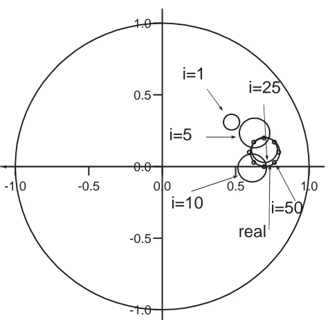
First we investigate the retrieval of an isotropic inclusion with conductivity k=10.0, i.e. k11=k22=10.0 and k12=k21=0.0 given by x0=0.7, y0=0.1 and r0=0.1. The convergence

(7)

-1.0 -0.5 0.0 0.5 1.0

i=1

i=5

i=50

i=10

i=25

[image:7.595.187.424.79.310.2]

real

Figure 1. The iterative convergence process as the best solution found by the GA moves towards the exact solution x0=0.7, y0=0.1, r0=0.1 for various numbers of generations

performed, namely i

∈

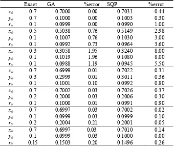
{1,5,10,25,50}, for the case of an isotropic inclusion with k=10.0 Table 1 presents the numerical results obtained for inclusions of various sizes and locations compared with the exact values and to the results obtained in Lesnic [17] by minimising the least squares functional (4) by a sequential quadratic programming (SQP) optimisation technique. By comparing the accuracy obtained for various sizes and locations of the inclusion, it can be seen that, as expected, larger inclusions are easier to detect than small inclusions and also inclusions located close to the surface Ω of the domain are easier to retrieve in comparison with equally sized inclusions located deep below the surface of the domain. It should be noted that the results obtained using the GA method are more accurate than those obtained with the SQP method. Moreover, the gradient based method may converge towards local optima, for particular initial guesses, while the GA was found to always retrieve the global optimum.

Retrieval of anisotropic inclusions

Next we consider an anisotropic inclusion D with a conductivity tensor given by









=

1

2

5

(8)

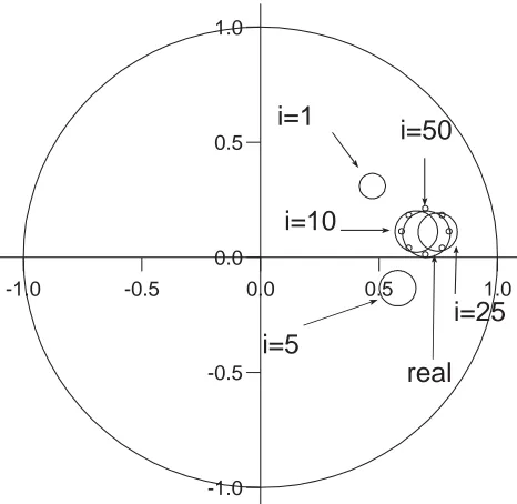
solution moves towards the real solution, is presented in Figure 2. Again it can be seen that the location and the size of the inclusion are accurately detected within 50 generations.

Exact GA %error SQP %error

x0 0.7 0.7000 0.00 0.7031 0.44

y0 0.7 0.1000 0.00 0.1003 0.30

r0 0.1 0.0999 0.00 0.0990 1.00

x0 0.5 0.5038 0.76 0.5149 2.98

y0 0.1 0.1007 0.76 0.1030 3.00

r0 0.1 0.0992 0.73 0.0964 3.60

x0 0.3 0.3058 1.95 0.3240 8.00

y0 0.1 0.1019 1.96 0.1080 8.00

r0 0.1 0.0988 1.19 0.0945 5.50

x0 0.7 0.6999 0.01 0.7022 0.31

y0 0.3 0.2999 0.01 0.3011 0.36

r0 0.1 0.1001 0.10 0.0992 0.80

x0 0.7 0.7002 0.03 0.7026 0.37

y0 0.2 0.2000 0.03 0.2006 0.30

r0 0.1 0.1000 0.01 0.0991 0.90

x0 0.7 0.6997 0.03 0.7002 0.02

y0 0.1 0.0999 0.03 0.0999 0.10

r0 0.2 0.2004 0.21 0.2001 0.05

x0 0.7 0.6997 0.03 0.7010 0.14

y0 0.1 0.0999 0.03 0.1000 0.00

[image:8.595.135.475.162.449.2]

r0 0.15 0.1503 0.20 0.1496 0.26 Table 1.The numerically retrieved values for the parameters characterising the position and the shape of an isotropic inclusion D with the conductivity k=10, for various positions and sizes of the inclusion, in comparison with the results obtained by minimising the object function (4) using a sequential quadratic programming (SQP) method.

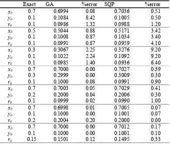
Table 2 presents the numerical results obtained for the parameters x_0, y_0 and r_0 in comparison with the results obtained in Mera and Lesnic [23] by minimising the least squares functional (4) by a sequential quadratic programming (SQP) optimisation technique. It should be noted that also in the anisotropic case the GA ourtperforms the SQP optimisation technique in most of the cases investigated.

(9)

Conclusions

In this paper the inverse conductivity problem which requires the determination of the location, size and/or non-dimensional anisotropic conductivity tensor, K, of a circular inclusion D contained in a domain Ω from measured electric voltage, φ, and electric current flux,

n

∂

∂ϕ

_{, on the boundary} _Ω_{has been investigated numerically using a}

GA. The results were compared with the results obtained using a SQP gradient based method. The GA was found to outperform the gradient based method. Overall, it may be concluded that the GA based method investigated is a robust, efficient method for detecting the size and location of subsurface inclusions.

Exact GA %error SQP %error

x0 0.7 0.6994 0.08 0.7036 0.51

y0 0.1 0.1084 8.42 0.1005 0.50

r0 0.1 0.0986 1.32 0.0988 1.20

x0 0.5 0.5044 0.88 0.5171 3.42

y0 0.1 0.1008 0.87 0.1034 3.40

r0 0.1 0.0991 0.87 0.0959 4.10

x0 0.3 0.3067 2.25 0.3276 9.20

y0 0.1 0.1022 2.24 0.1092 9.20

r0 0.1 0.0985 1.40 0.0936 6.40

x0 0.7 0.7000 0.00 0.7027 0.39

y0 0.3 0.2999 0.00 0.3009 0.30

r0 0.1 0.1000 0.08 0.0991 0.90

x0 0.7 0.7003 0.05 0.7029 0.41

y0 0.2 0.2000 0.04 0.2006 0.30

r0 0.1 0.0999 0.02 0.0990 1.00

x0 0.7 0.6998 0.01 0.7005 0.07

y0 0.1 0.1000 0.00 0.1001 0.07

r0 0.2 0.2004 0.20 0.2000 0.00

x0 0.7 0.7000 0.00 0.7012 0.17

y0 0.1 0.1000 0.00 0.1001 0.10

[image:9.595.136.475.281.569.2]

(10)

sizes of the inclusion, in comparison with the results obtained by minimising the object function (4) using a sequential quadratic programming (SQP) method.

-1.0 -0.5 0.0 0.5 1.0

i=1

i=5

i=25

i=10

i=50

[image:10.595.187.420.132.359.2]

real

Figure 2. The iterative convergence process as the best solution found by the GA moves towards the exact solution x0=0.7, y0=0.1, r0=0.1 for various numbers of generations

performed, namely i

∈

{1,5,10,25,50}, for the case of an anisotropic inclusion with k11=5.0,

k12=2.0 and k22=1.0.

REFERENCES

[1]M. Lee and G. Uhlmann, Determining anisotropic real-analytic conductivities by boundary measurements, Commun. Pure Appl. Math., 42, 1097-1112, (1989). [2]J. Sylvester, An anisotropic inverse boundary value problem, Commun. Pure Appl. Math 43, 201-232, (1990).

[3]W.R.B. Lionheart, Conformal uniqueness results in anisotropic electrical impedance imaging, Inverse Problems 13, 125-134, (1997)

(11)

[6]J.K. Seo, On the uniqueness in the inverse conductivity problem, J. Fourier Anal. Appl 2, 227-235, (1996).

[7]H. Kang and J.K. Seo, The layer potential technique for the inverse conductivity problem, Inverse Problems 12, 267-278, (1996).

[8]F. Hettlich and W. Rundell, The determination of a discontinuity in a conductivity from a single boundary measurement, Inverse Problems14, 67-82,(1998).

[9]G. Alessandrini and V. Isakov, Analyticity and uniqueness for the inverse conductivity problem, Rend. Istit. Mat. Univ. Trieste 28, 351-369,(1996).

[10]M. Ikehata, On reconstruction in the inverse conductivity problem with one measurement, Inverse Problems 16, 785-793, (2000)

[11]V. Isakov, On uniqueness of recovery of a discontinuous coefficient, Commun. Pure Appl. Math. 41, 865-877, (1988)

[12]M. Ikehata, Size estimation of inclusion, J. Inv. Ill-Posed Problems 6, 127-140, (1998).

[13]M. Ikehata, G. Nakamura and K. Tanuma, Identification of the shape of the inclusion in the anisotropic elastic body, Appl. Anal. 72, 17-26, (1999).

[14]N.S. Mera, L. Elliott and D.B. Ingham, Detection of subsurface cavities in IR-CAT by a real coded genetic algorithm, Applied Soft Computing, in print

[15]D.E. Goldberg, Genetic Algorithm in Search, Optimisation and Machine Learning}, Addison-Wesley, Reading, (1989).

[16]Z. Michalewicz, Genetic Algorithms + Data Structures = Evolution Programs, 3rd Edn., Springer-Verlag, Berlin, (1996).

[17]D. Lesnic, A numerical investigation of the inverse potential conductivity problem in a circular inclusion, Inverse Problems in Engineering 9, 1-17, (2001). [18]O.A. Ladyzhenskaya The Boundary Value Problems of Mathematical Physics, Springer-Verlag, Berlin, (1985).

[19]Y.P. Chang, C.S. Kang and D.J. Chen, The use of fundamental Green's functions for the solution of heat conduction in anisotropic media, Int. J. Heat Mass Transfer 16, 1905-1918, (1973).

[20]N.S. Mera, L. Elliott, D.B. Ingham and D. Lesnic, The boundary element solution of the Cauchy steady heat conduction problem in an anisotropic medium, Int. J. Numer. Meth. Eng. 49, 481-499, (2000).

[21]H. Kang and J.K. Seo, Identification of domains with near-extreme conductivity: global stability and error estimates, Inverse Problems 15, 851-867, (1999).

[22]H. Kang and J.K. Seo, Identification of domains with near-extreme conductivity: global stability and error estimates, Inverse Problems 15, 851-867, (1999).

(12)

[24]Mera, N.S., Elliott, L. and Ingham, D.B., A real coded genetic algorithm approach for subsurface isotropic and anisotropic inclusions detection, Inverse Problems in Engineering, in print.

Authors:

N.S. Mera-Centre for Computational Fluid Dynamics, University of Leeds, Leeds, LS2 9JT, United Kingdom

L. Elliott- Department of Applied Mathematics, University of Leeds, Leeds, LS2 9JT, United Kingdom