Paul Sullivan and Ted To are research economists at the U.S. Bureau of Labor Statistics. The authors thank Timothy Erickson, Kuo- Liang Chang, Loren Smith, two anonymous referees, and seminar participants at Georgetown University, the U.S. Census Center for Economic Studies, the 2010 Western Economic Association Meeting, and the 2012 ASSA Meeting for helpful comments. Discussant comments from Peter Arcidiacono were particularly helpful. The views expressed are those of the authors and do not necessar-ily refl ect those of the Bureau of Labor Statistics. The data used in this article can be obtained beginning October 2014 through September 2017 from Paul Sullivan or Ted To, Bureau of Labor Statistics, Postal Square Building, 2 Massachusetts Ave. N.E., Washington, D.C. 20212; Sullivan.Paul.Joseph@bls .gov, To.Theodore@bls .gov.
[Submitted September 2011; accepted May 2013]
ISSN 0022- 166X E- ISSN 1548- 8004 © 2014 by the Board of Regents of the University of Wisconsin System
T H E J O U R N A L O F H U M A N R E S O U R C E S • 49 • 2
Characteristics
Paul Sullivan
Ted To
A B S T R A C T
This paper quantifi es the importance of nonwage job characteristics to workers by estimating a structural on- the- job search model. The model generalizes the standard search framework by allowing workers to search for jobs based on both wages and job- specifi c nonwage utility fl ows. Within the structure of the search model, data on accepted wages and wage changes at job transitions identify the importance of nonwage utility through revealed preference. The estimates reveal that utility from nonwage job characteristics plays an important role in determining job mobility, the value of jobs to workers, and the gains from job search.
I. Introduction
Nonwage job characteristics are important determinants of job mo-bility and choice. Important nonwage job characteristics include employer provided health insurance (Gruber and Madrian 2004), employer provided retirement benefi ts,
fl exible hours (Altonji and Paxson 1992), paid vacation, occupational choice (God-deeris 1988), risk of injury or death (Thaler and Rosen 1975), commuting time (White 1988), onsite amenities, or a whole host of other, possibly intangible or heteroge-neously valued,1 job characteristics. Despite their importance, there is relatively little research that estimates search models with nonwage job characteristics and studies
their effect on job choice and mobility decisions. The bulk of the empirical search literature assumes that the wage captures the entire value of a job and the literature that does account for nonwage job characteristics typically focuses on a single job char-acteristic. For example, Blau (1991), Bloemen (2008), Flabbi and Moro (2010), and Gørgens (2002) estimate models with hours or hours fl exibility, Dey and Flinn (2005, 2008) estimate models with health insurance provision, and Sullivan (2010) estimates a model with occupational choice. Instead of focusing on a single observable job char-acteristic, we estimate a structural search model that allows workers to derive utility from their aggregate valuation of all the nonwage characteristics of a particular job.
The goals of this paper are to estimate the total value that workers place on the non-wage attributes of their jobs and to quantify the importance of nonnon-wage factors in de-termining individual labor market dynamics. To accomplish this, we estimate a search model which augments the standard income maximizing on- the- job search framework (Burdett 1978) by including utility from nonwage job characteristics. In the model, employed and unemployed workers search across jobs that offer different wages and levels of nonwage utility. When a worker and fi rm meet, the worker receives a wage offer and also observes a match- specifi c nonwage utility fl ow that represents the net value that this particular worker places on all the nonwage job characteristics pres-ent at the job. Search frictions are prespres-ent because both job offers and layoffs occur randomly, and because both wages and nonwage match values are modeled as random draws from a distribution that is known to the worker. Following a large fraction of the empirical search literature, we adopt a stationary, partial equilibrium framework.2 As in the canonical on- the- job search model, wage growth occurs as workers climb a job ladder by moving to higher wage jobs. A novel feature of the model is that it also allows workers to benefi t from moving to jobs that offer higher nonwage utility. Depending on the importance of the nonwage side of the model, basing conclusions about the value of job mobility solely on wages could give a misleading view of the gains to job search and mobility. Estimating the structural model is a direct way of quantifying the importance of the wage and nonwage channels in determining the total gains to mobility over the career.
The structural parameters are estimated by simulated minimum distance using the 1997 cohort of the National Longitudinal Survey of Youth (NLSY97). The estimates reveal that workers place a substantial value on nonwage job characteristics, and also show that nonwage utility fl ows vary widely across different worker- fi rm matches. More specifi cally, workers who are searching for a job face slightly more dispersion in job- specifi c nonwage utility fl ows than in wage offers. Simulations performed us-ing the estimated model reveal that increases in the utility derived from nonwage job characteristics account for approximately one- half of the total gains from job mobility. This result indicates that standard models of on- the- job search—which are based solely on wages—are missing a key determinant of the value of jobs, the causes of worker mobility, and the gains from job search.
Our use of the nonwage match value as an aggregate measure of the nonwage value of a job is primarily motivated by the goal of estimating the total nonwage value of jobs to workers. In addition, four observations about the information available in
standard sources of labor market data on the employer provided benefi ts, tangible job characteristics, and intangible job characteristics that differentiate jobs are relevant. First, important employer provided benefi ts such as health insurance and retirement plans are imperfectly measured.3 Second, information about many tangible job char-acteristics, such as risk of injury or commuting time, is frequently unavailable. Third, measures of intangible job characteristics such as a worker’s evaluation of his supervi-sor, which may be signifi cant determinants of the value of a job to a worker, are typi-cally completely absent. Fourth, and perhaps most importantly, it is likely that workers have heterogeneous preferences over the employer provided benefi ts and tangible and intangible job characteristics that differentiate jobs. With these facts in mind, rather than attempting to estimate the value of specifi c job characteristics, we estimate the net value of all nonwage job characteristics to a worker using the nonwage match value.
This paper contributes to a growing literature that demonstrates the importance of accounting for imperfect information, search frictions, and dynamics when estimat-ing the value of nonwage job characteristics. Hwang, Mortensen, and Reed (1998), Dey and Flinn (2005, 2008), and Gronberg and Reed (1994) all discuss the problems caused by using a static framework to analyze nonwage job characteristics in a dy-namic labor market. More recently, Bonhomme and Jolivet (2009) estimate the value of a number of observed job characteristics using a search model. We take a different approach by estimating the total nonwage value of jobs using the nonwage match value, rather than attempting to identify the value of specifi c characteristics. Becker (2010) develops a model that focuses on incorporating nonwage utility into the equi-librium wage bargaining framework of Postel- Vinay and Robin (2002) and applying the model to unemployment insurance.
Nonwage utility fl ows are of course not observed by the econometrician so identifi -cation is an important concern. The on- the- job search model provides a natural frame-work for using data on wages, job acceptance decisions, and employment durations to infer the value that workers place on nonwage job characteristics. Broadly speaking, the intuition behind the identifi cation of the model is that since a standard income maximizing search model is nested within the utility maximizing search model, the importance of nonwage job characteristics is identifi ed by the extent to which an in-come maximizing model fails to explain the moments used in estimation. More specif-ically, observed patterns of job mobility and wage changes at transitions between jobs are particularly informative about the importance of nonwage job characteristics. To give a concrete example, a key moment matched during estimation is the proportion of direct job- to- job transitions where workers choose to accept a decrease in wages.4 Wage declines at job transitions occur frequently: In the NLSY97 data, reported wages decline for more than one- third of direct transitions between jobs. Taking the structure of the model as given, this type of transition indicates through revealed preference that a worker is willing to accept lower wages in exchange for higher nonwage utility at a specifi c job.
3. For example, in the 1979 and 1997 cohorts of the NLSY, information is available about whether or not employers offer benefi ts such as health insurance but there is no information about takeup of benefi ts, dollar amount of the employer and employee contributions, or plan quality.
During estimation, we are careful to account for the two alternative explanations for observed wage decreases at direct transitions between jobs that have dominated the empirical search literature up to this point. Ignoring either of these possible explana-tions during estimation would lead to an upward bias in the estimated importance of nonwage utility. The fi rst explanation is that if a job ends exogenously, a worker might choose to move directly to a lower- paying job to avoid unemployment, if this option is available.5 The second explanation is that measurement error in wages might cause some transitions between jobs that are actually accompanied by wage increases to be erroneously shown as wage decreases in the data.6 Our model allows for both of these explanations, and also adds a third possible explanation: A worker could choose to move from a high- wage job to a lower- wage job that offers a higher level of nonwage utility.
We incorporate the involuntary direct transitions into the model by allowing exist-ing jobs to end involuntarily (from the perspective of the worker) in the same time period that a job offer is received from a new employer. The probability that this event occurs is identifi ed using NLSY97 data that identifi es direct job- to- job transitions that begin with involuntary job endings. Existing research has not used this type of data to identify involuntary direct transitions between employers.
We account for measurement error in wages by estimating a parametric model of measurement error jointly along with the other parameters of the model. Although at
fi rst glance it might appear that measurement error in wages and match- specifi c non-wage utility are observationally equivalent, Section IV.D of this paper demonstrates that they actually have very different implications for the simulated moments used to estimate the model. More specifi cally, although measurement error and nonwage util-ity can both account for observed wage decreases at job transitions, neither feature on its own is capable of simultaneously explaining the extent of variation in wages, the amount of wage growth over the career, and the frequency of wage declines at direct job transitions in the NLSY97.
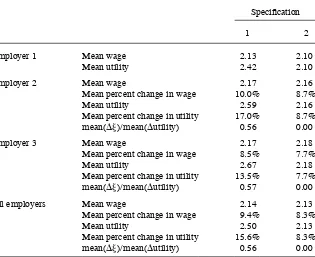
The parameter estimates reveal that the variation in nonwage utility fl ows across worker- fi rm matches is slightly greater than the variation in wage offers. This implies that there are substantial gains to workers from job search based on nonwage factors. Although the parameter estimates provide direct evidence on the importance of the nonwage side of the model, perhaps a more informative way of examining the impli-cations of the utility maximizing search model is to study simulated data generated by the estimated model. In these data, nonwage utility accounts for 23 percent of the total variation in the one- period utility fl ows that workers receive from employment. On average, measuring the value of a job using only the wage substantially under-states the true value of a job to a worker. More specifi cally, in 85 percent of all jobs in the simulated data, workers value the nonwage characteristics of their job greater than the mean offered value of nonwage job characteristics. The fact that workers receive below mean nonwage utility fl ows in only 15 percent of accepted job offers
5. For example, Jolivet, Postel- Vinay, and Robin (2006) assume that all direct job- to- job transitions accom-panied by wage decreases are the result of simultaneous job endings and mobility to new jobs.
shows that although utility maximizing workers in the model are perfectly willing to accept higher wages in exchange for undesirable job characteristics, the search model reveals a strong tendency for workers to sort into jobs with nonwage job char-acteristics that they are willing to pay for. The above average nonwage value of jobs is generated by two features of the search environment. First, the reservation utility strategy followed by unemployed agents implies that the accepted job offers observed in the simulated data are truncated from below. Second, on- the- job search implies that workers climb both wage and nonwage utility ladders as they move between employers.
The search model with nonwage job characteristics has important implications for the study of compensating differentials. Previously, papers such as Hwang, Mortensen, and Reed (1998) and Gronberg and Reed (1994) make the point that in general, es-timates of compensating differentials will be biased unless search frictions are taken into account. Our primary contribution to this line of research is to use the estimated structural search model to obtain a direct estimate of the magnitude of the bias caused by estimating compensating differentials using a static framework. Standard hedonic regression approaches to valuing nonwage job characteristics implicitly assume that workers are free to select an optimal job from a perfectly known labor market he-donic wage curve. In contrast, the simulated data from our model contain a sample of wages and nonwage utility received by workers who must search for jobs in a dynamic labor market due to imperfect information about available job opportunities. When we estimate a standard hedonic regression using these data, the estimated willingness- to- pay for nonwage job characteristics is biased downward by approxi-mately 50 percent from the true value used to generate the data.
This application of the model offers an explanation for the fact that empirical sup-port for the theory compensating differentials is relatively weak, despite a vast lit-erature on estimating these differentials. The intuition behind the downward bias in estimated compensating differentials is that in a search model, the only information provided by accepted pairs of wages and nonwage utility is that they exceed a reserva-tion utility threshold. In this setting, they do not directly reveal the marginal willing-ness to pay for nonwage job characteristics as they would in a static, frictionless, perfect information world where workers maximize utility subject to a given labor market hedonic wage locus.
In the following section, we develop a partial equilibrium model of on- the- job search with nonwage utility. In Section III, we discuss the data set used to estimate our model and in Section IV we discuss our econometric methodology and some important identifi cation issues. Section V presents our parameter estimates and discusses the effect of nonwage utility on labor market outcomes. Section VI concludes.
II. The Search Model with Utility from Nonwage Job
Characteristics
unemploy-ment.7 Agents randomly receive job offers while unemployed and employed, and the employed face a constant risk of exogenous job loss.8 When a job ends exogenously, there is no chance of recall. For ease of exposition, this section describes the decision problem facing a single agent. However, we allow for person- specifi c unobserved heterogeneity when estimating the model (Section IV).
A. Preferences and job offers
The utility received by an employed agent is determined by the log- wage, w, and the match- specifi c nonwage utility fl ow, ξ. The one- period utility from employment is
(1) U(w,ξ) = w + ξ,
where both w and ξ are specifi c to a particular match between a worker and employer, and are constant for the duration of the match. A job offer consists of a random draw of (w,ξ) from the distribution F(w,ξ), which is a primitive of the model. Although with this functional form, the saving decision is no longer irrelevant as it is with the linear utility functions that are commonly adopted in search models, it has the desirable property that the marginal utility of the wage declines as the wage increases—this is particularly important for our application because the tradeoff between wages and nonwage utility is central to the workers’ mobility decisions. While explicitly allowing savings in our model would be of interest in its own right, it is beyond the scope of our current exercise and we leave it as an extension for future research.
The structure of the search and matching process in the model labor market is as fol-lows. When a worker and fi rm randomly meet, the worker receives a wage offer. At the same time, the worker observes the complete bundle of nonwage job characteristics present at the fi rm. These characteristics include employer provided benefi ts (health insurance), tangible job characteristics (risk of injury, commuting time), and intangible job characteristics (friendliness of coworkers). Based on his preferences, which may be heterogeneous across agents, the worker determines the net value of the nonwage job characteristics present at this fi rm (ξ).9 The worker then decides whether or not to accept the job offer. Once a job offer is accepted, the wage and nonwage component of the offer remain constant for the duration of the job spell.10 Because our primary goal is to estimate the total importance of nonwage job characteristics to workers, which is captured by ξ, we do not attempt to determine how much of the variation in nonwage
7. Following the majority of the search literature, the model does not distinguish between unemployment and nonparticipation in the labor market.
8. The terms exogenous job endings and layoff are used interchangeably in the remainder of the paper. 9. One specifi c nonwage job characteristic that is likely to be refl ected in ξ is hours of work. (See Blau 1991 and Bloemen 2008 for search models which focus on hours.) However, the utility function shown in Equa-tion 1 is separable in its two arguments, which rules out interacEqua-tions between w and ξ—which may be im-portant in a model where hours of work are explicitly modeled. Also, it is worthwhile to note that we restrict our analysis to full- time jobs (Section III) so hours only vary in our sample to the extent that they vary within full- time jobs. The primary advantage of our separable utility function is that it provides a straightforward, tractable framework for thinking about how workers evaluate jobs that differ in (w, ξ). It is also consistent with existing literature on search with nonwage amenities such as Dey and Flinn (2005). Of course, it is less general than other possible functional forms.
utility is due to fi rm level variation in nonwage job characteristics versus preference heterogeneity.11
B. Unemployed search
Unemployed agents search for jobs, which arrive randomly with probability λu. Since w
and ξ are additively separable in the utility function, it is convenient to defi ne the agent’s decision problem in terms of total utility, w + ξ, where U(w,ξ) ≡U and U is distributed as H(U). Note that the distribution function H(·) is not a primitive of the model and is derived from the joint distribution function for log- wages and nonwage utility. In particular, if the joint distribution is F(w, ξ) then H(U)=∫
−∞ ∞ F
w|(U−|)f()d
where Fw|ξ is the cumulative conditional wage distribution and fξ is the unconditional probability density function for ξ. The discounted expected value of lifetime utility for an unemployed agent is
(2) Vu=b+␦[
uEmax{V u
,Ve(U′)}+(1−
u)V u
],
where b is the one- period utility fl ow from unemployment, which refl ects the value of unemployment benefi ts and leisure, and δ is the discount factor. The term Ve(U′) represents the expected discounted value of lifetime utility for an agent employed in a job with utility level U′.
The optimal search strategy for an unemployed agent is a reservation utility strat-egy, which is analogous to the reservation wage strategy found in income maximizing search models. The rule is to accept any job offer which offers a one- period utility
fl ow greater than the reservation level, U*, and reject all other offers. Appendix 1 presents the formal derivation of U*. This stationary unemployed search problem as-sumes away duration dependence in unemployment spells. A large empirical literature examines duration dependence in unemployment spells.12 In the NLSY97 data used to estimate the model, the hazard rate out of unemployment is approximately constant so the constant exit rate assumed by the model is broadly consistent with the data.13
C. On- the- job search
In each time period, with probability λe an employed agent receives a job offer from an outside fi rm. The worker may accept the job offer, or reject it and continue working for his current employer. Job matches end with exogenous probability λl. When a job ends for this reason, the worker is forced to become unemployed. With probability
11. We leave decomposing the sources of variation in match- specifi c nonwage utility as an interesting, although diffi cult, extension for future research. Empirical work along these lines would require detailed data on the complete set of nonwage job characteristics valued by workers along with suffi ciently high mobility rates between jobs with different characteristics to identify preference heterogeneity. In addition, data on the
fi rm side of the market, ideally matched worker- fi rm data, would be useful to control for unobserved, fi rm- specifi c variation in working conditions and job amenities.
λle, a worker’s current job exogenously ends and he receives a job offer from a new employer in the same time period. When this happens, the worker can accept the new offer or become unemployed. Finally, with probability (1 – λe – λl – λle) the job does not end exogenously and no new offers are received, so the worker remains in his current job.
The discounted expected value of lifetime utility for a worker who is currently employed in a job with utility level U is
(3) Ve(U)=U+␦[eEmax{Ve(U),Ve(U′)}+lVu +
leEmax{V
u,Ve(U′)}+(1−
e−l−le)V e(U)]
The fi rst term within the square brackets in Equation 3, λeEmax{Ve(U),Ve(U′)}, repre-sents the expected value of the best option available in the next time period for an em-ployed individual who receives a job offer from a new employer.14 The second brack-eted term, λlVu, corresponds to the case where a job exogenously ends and the worker is forced to enter unemployment. The third bracketed term, λleEmax{Vu,Ve(U′)}, rep-resents the case where the worker is laid off but also receives a job offer from a new employer. The fi nal bracketed term represents the case where the worker is neither laid off nor receives an outside job offer.
In this stationary search environment, optimal decisions for employed agents are based on comparisons of one- period utility fl ows. When an employed agent receives an offer from an outside fi rm but does not experience an exogenous job ending, a simple reservation utility strategy is optimal. Because Ve(U) is increasing in U, the rule is to accept the offer if it offers greater utility than the current job (U′ > U), and reject the offer otherwise (U′≤U). If a worker’s job exogenously ends and he receives a new job offer at the same time, which occurs with probability λle, the situation is identical to the one faced by an unemployed agent who receives a new job offer. As a result, he will choose to accept or reject the offer based on the unemployed reservation utility level U*.
In the remainder of the paper, we will refer to direct job- to- job transitions that occur as the result of a simultaneous layoff and job offer as “involuntary” transitions between employers. This terminology refl ects the fact that although a direct job- to- job transition occurs, the worker’s previous job ended involuntarily (exogenously). For agents in the model, voluntary and involuntary transitions are fundamentally different types of job mobility. When a voluntary job- to- job transition occurs, utility increases (U′ > U). In contrast, when an involuntary transition occurs, the new job offer is pref-erable to unemployment (U′ > U*), but it may be the case that total utility is lower than the previous job that exogenously ended (U′ < U).
III. Data
We use the 1997 rather than the venerable 1979 cohort of the NLSY to estimate our model for two reasons. First, the NLSY97 is more representative of
rent labor market conditions. Second, the NLSY97 design team incorporated lessons from the NLSY79 and has a more consistent methodology (Pergamit et al. 2001).
The NLSY97 is a nationally representative sample of 8,984 individuals who were between the ages of 12 and 16 on December 31, 1996. Interviews have been conducted annually since 1997. The NLSY97 collects extensive information about labor market behavior and educational experiences that provide the information needed to study the transition from schooling to employment, early career mobility between employers, and the associated dynamics of wages. Individuals enter the estimation sample when they stop attending high school. The information from the annual interviews is used to construct a weekly employment record for each respondent.
We select a particular subset of the NLSY97 in order to minimize unnecessary com-plications in estimating our model. Women are excluded for the usual reason of avoid-ing the diffi culties associated with modeling female labor force participation. Similarly, in order to avoid issues relating to household search, men who are ever married during the sample period are excluded. Moreover, we use data from interviews up to the 2006 interview and we select workers who have never attended college because low- skilled workers with little work experience can be expected to have little or no bargaining power and hence conform best to our wage- posting model. Thus we focus on young, unmarried, low- skilled men who are at the beginning of their careers. As is standard in the empirical search literature, individuals who ever serve in the military or are employed are excluded from the sample. Because the maximum age that an individual could reach during the sample period is only 26 years, our results should be viewed as applying to young workers who tend to be quite mobile during this early phase of their career. Whether the results generalize to older workers, or different cohorts of workers, is an open question.
The NLSY97 provides a weekly employment record for each respondent that is aggregated into a monthly15 labor force history for the purposes of estimation. First, each individual is classifi ed as unemployed or employed full- time16 for each month depending on whether more weeks were spent employed or unemployed during the month.17 Next, employed individuals are assigned a monthly employer based on the employer that the worker spent the most weeks working for during the month. The monthly wage is the one associated with the monthly employer. The monthly employ-ment record contains a complete record of employemploy-ment durations, direct transitions between employers that occur without an intervening spell of unemployment, transi-tions into unemployment, and the growth in wages resulting from mobility between employers.
Since the importance of nonwage job characteristics is identifi ed in part by job- to- job transitions, we are careful to differentiate between those that are voluntary and those that are not. To identify involuntary job- to- job transitions we use the stated reason that a worker left their job. We consider “layoffs,” “plant closings,” “end of
15. For tie- breaking purposes, we use a fi ve- week month.
16. We classify full- time employment as 15 or more hours per week. Individuals working less than 15 hours per week are classifi ed as unemployed. In our data, unemployment spells involving part- time work make up only 5.3 percent of all unemployment spells.
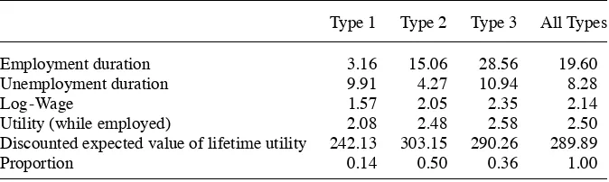
a temporary or seasonal job,” “discharged or fi red,” or “program ended” to be invol-untary. While these data may be somewhat noisy, we are reassured by the summary statistics that show that direct transitions we classify as strictly involuntary are more likely to result in a wage decline (Table 1). In addition, on average, workers who make involuntary transitions between employers experience nearly a 2 percent decline in wages. In contrast, wages increase on average by 8 percent at all transitions between employers.
The fi nal issue worthy of discussion regarding the data is the treatment of within- job variation in wages. In the NLSY97, when a job persists across survey interviews, which occur approximately one year apart, a new measurement of the wage is taken. If a job does not last across interview years, only the initial measurement of the wage is available. In principle, it would be possible to allow for within- job variation in wages using these data. However, as discussed by Flinn (2002), jobs with observed wage changes are not a random sample from the population, so there are diffi cult selection issues that must be confronted when estimating an on- the- job wage process using these data. Even more importantly for our purposes, since the NLSY97 is still a relatively short panel, the majority of jobs do not persist across survey years. For these jobs, it is impossible to observe on- the- job wage growth; we only observe a single wage for 72 percent of all jobs in our data. To be precise, for our estimation sample we are unable to reject the null hypothesis that mean wage growth is zero within job spells.18 Given these features of the data, there is little hope of precisely estimating an on- the- job wage growth process. As a result, we restrict wages to be constant within job spells for the purposes of estimation. When multiple wages are reported for a particular job, we use the fi rst reported wage as the wage for the entire job spell. Moreover, for our application, with our focus on young, unskilled workers during the highly mobile, early stage of their career, constant wages within jobs does not seem unrealistic.
A. Descriptive statistics
This section highlights the key characteristics of the data used to estimate the im-portance of nonwage job characteristics in determining employment outcomes. It is convenient to describe the labor market histories in the data and the data generated by the search model in terms of employment cycles, as in Wolpin (1992). An employment cycle begins with unemployment and includes all of the following employment spells that occur without an intervening unemployment spell. When an individual enters unemployment, a new cycle begins. In the remainder of the paper, whenever a job is referred to by number, it represents the position of the job within an employment cycle.
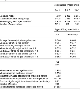
Table 1 shows the means and standard deviations of key variables from the sample of the NLSY97 used in this analysis. There are 980 individuals in the data who remain in the sample for an average of 54.2 months, and these people experience an average
Table 1
Descriptive Statistics: NLSY97 Data
Job Number Within Cycle
Job 1 Job 2 Job 3
Mean log- wage 1.979 2.038 2.061
Standard deviation of log- wage 0.425 0.458 0.457
Mean employment spell durationa 8.939 9.271 9.738
Number of observations 2614 940 382
Type of Employer Switch
All Involuntary
Pr(wage decrease) at job- to- job move 0.364 0.460
Mean ∆w at job- to- job switchb 0.081 –0.017
Median ∆w at job- to- job switch 0.074 0.000
Mean ∆w at job- to- job switch |∆w > 0 0.359 0.322
Median ∆w at job- to- job switch |∆w > 0 0.231 0.211
Mean ∆w at job- to- job switch |∆w < 0 –0.327 –0.345
Median ∆w at job- to- job switch |∆w < 0 –0.163 –0.206
All Jobs
Mean unemployment spell duration 5.908
Mean number of cycles per personc 2.878
Standard deviation of number of cycles per person 1.793 Mean total work experience at end of sample periodd 40.010 Fraction of job- to- job transitions that are involuntary 0.151
Number of people 980
Mean number of months in sample per person 54.153
Notes: a. All durations are measured in months.
b. ∆w represents the change in the wage at a job- to- job transition.
c. An employment cycle begins with the fi rst job after an unemployment spell, and includes all subsequent jobs that begin without an intervening unemployment spell.
of 2.88 employment cycles. The top section of the table shows that as individuals move between employers within an employment cycle, the average wage and employ-ment duration increase.19 The middle section of the table shows that although mean wages increase as individuals move directly between jobs, conditional on switching employers without an intervening unemployment spell there is a 36 percent chance that an individual reports a lower wage at his new job.20 For individuals who report that the direct transition between employers was involuntary, the mean wage change is negative, and the probability of a wage decrease rises to 46 percent. Measurement error in wages certainly accounts for some fraction of the observed wage decreases at voluntary transitions between employers. However, the prevalence of these wage decreases and the increased probability of observing a wage decline at an involuntary transition both suggest a role for nonwage job characteristics in determining mobility between jobs.
We conclude our analysis of the data with a discussion of the extent to which two important features of the search model are consistent with the patterns found in the NLSY97 data. First, the model assumes that workers who experience an involuntary job ending draw new job offers from the same distribution as unemployed workers. In reality, it may be the case that workers receive prior notice of job endings, and respond by increasing their on- the- job search effort. Because search effort is unobserved, we compare the observable characteristics of jobs that begin with an involuntary job end-ing to those of jobs that begin with a transition from unemployment. In the NLSY97 data, the average log- wage on jobs that begin with an involuntary job- to- job transition is only 0.005 lower than the average wage on jobs that begin with a transition from unemployment. Similarly, on average, a job that begins with an involuntary transition lasts only two weeks less than a job that begins with a transition from unemployment. Based on these statistics, assuming that the unemployed and involuntarily displaced draw job offers from the same distribution seems to be broadly consistent with the data. Second, the omission of general human capital implies that in the model, wages will not grow across employment cycles. In the NLSY97 data, the mean growth in wages between Job 1 in Employment Cycle 1 and Job 1 in Employment Cycle 2 is 0.1396 with a t- statistic of 0.2889. While the magnitude of this wage growth appears to be large, it is not statistically distinguishable from zero.
IV. Estimation
The parameters of the model are estimated by simulated minimum dis-tance (SMD). This section begins by specifying the distributional assumptions about the job offer distribution, measurement error in wages, and unobserved heterogeneity needed to estimate the model. Then it explains how the simulated data is generated, describes the estimation algorithm, and discusses identifi cation.
19. Statistics are not reported for more than three jobs within a cycle because only a very small number of people have four or more consecutive jobs without entering unemployment.
A. Distributional assumptions
1. The wage offer distribution
Estimating the model requires specifying the distribution F(w,ξ), which is a primitive of the model.21 We assume that log- wage offers and match- specifi c utility fl ows are independent, and normally distributed,22
(4) F(w,ξ) ~ Ω(w)Ψ(ξ)
(5) Ω(w) ~ N(μw,σw)
(6) Ψ(ξ) ~ N(0,σξ)
Note that our normalization of the mean nonwage utility offer to zero is an innocuous assumption because, as in any discrete choice model, utility fl ows are only identifi ed relative to a base choice. We normalize the employment nonwage utility fl ow to zero and estimate b, the nonpecuniary utility fl ow from unemployment.23
2. Measurement error in wages
A large literature surveyed by Bound, Brown, and Mathiowetz (2001) fi nds that wages in typical sources of microeconomic data are measured with error. We account for measurement error by assuming that the relationship between the log- wage observed in the data and the true log- wage is wo = w + ε, where wo is the observed log- wage,
w is the true log- wage, and ε ~ N(0,σε) represents measurement error in wages that is independent of the true wage.24 The parameter σ
ε is estimated jointly along with the other parameters in the model. Section IV.D discusses how the extent of measurement error in wages is separately identifi ed from the importance of nonwage utility. The addition of measurement error in wages to the model does not change the optimiza-tion problem faced by agents because optimal decisions are based on true wages, not observed wages. However, measurement error impacts the simulated data used to estimate the model.
3. Accounting for unobserved heterogeneity
The search model presented in Section II assumes that all individuals are ex ante
identical at the start of their careers, which implies that all differences in wages and employment outcomes are driven by randomness in the labor market. Although the
21. We do not attempt to endogenize the job offer distribution because our primary goal in this paper is to quantify the relative importance of nonwage utility for workers, taking the offer distribution as given. Devel-oping a tractable partial equilibrium model allows us to focus directly on this issue, as in much of the existing literature that uses search models to quantify the monetary gains to search and mobility (Jolivet, Posel- Vinay, and Robin 2006; Flinn 2002; Sullivan 2010).
22. The latter part of Section IV.D discusses the assumed independence of w and ξ within the context of identifi cation.
23. An observationally equivalent model instead normalizes b to 0 and allows the mean nonwage utility offer to be a free parameter.
sample of workers from the NLSY97 used in estimation consists of a fairly homo-geneous group in terms of observable characteristics, it is possible that there are permanent differences between workers that are unobserved to the econometrician. In general, ignoring unobserved heterogeneity during estimation will lead to biased parameter estimates if unobserved heterogeneity is actually present.
In this application, the specifi c concern is that ignoring unobserved differences be-tween workers could lead to an overstatement of the importance of nonwage utility. For example, suppose that a worker remains in a job with a wage in the bottom 5 per-cent of the wage distribution over the entire sample period. If workers are assumed to be homogeneous, then the model will tend to explain the long duration of this low- wage job as a situation where the worker has a large draw of ξ, so he is willing to remain in the low- wage job because it provides a high level of utility. However, if there is heterogeneity across workers in ability, low- ability workers could choose to remain in jobs that offer low wages relative to the overall wage distribution because these jobs are actually high paying relative to their personal (low- ability) wage dis-tribution.
We account for person- specifi c unobserved heterogeneity in ability by allowing the mean of the wage offer distribution (μw) to vary across workers. Heterogeneity in preferences for leisure is captured by allowing the one- period utility fl ow from unem-ployment (b) to vary across workers. In addition, we allow the job offer arrival rates while unemployed (λu) and employed (λe), the layoff probability (λl), and the simulta-neous layoff- offer probability (λle) to vary across workers to allow for the possibility that workers face different amounts of randomness in job offer arrivals and exogenous job endings.25 Equation 8 shows that variation in these primitive parameters across workers leads to heterogeneity in the reservation utility level, U* across workers. Fol-lowing Keane and Wolpin (1997), and a large subsequent literature, we assume that the joint distribution of unobserved heterogeneity is a mixture of discrete types. As-sume that there are J types of people in the economy, and let pj represent the propor-tion of type j in the population. The parameters of the distribution of unobserved het-erogeneity, {w(j),b(j),u(j),l(j),e(j),le(j),j}j=1
J , are estimated jointly along
with the other parameters of the model.
B. Data simulation
As discussed in Section II, the optimal decision rules for the dynamic optimization problem can be described using simple static comparisons of one- period utility fl ows. It is straightforward to simulate data from the model using these optimal decision rules without numerically solving for the value functions that characterize the optimization problem.
The fi rst step when simulating the model is to randomly assign each individual in the data to one of the J discrete types that make up the population distribution of unobserved heterogeneity. Next, a simulated career is formed for each individual in the NLSY97 estimation sample by randomly generating job offers and exogenous job endings, and then assigning simulated choices for each time period based on the
ervation value decision rules. The number of time periods that each simulated person appears in the simulated data is censored to match the corresponding person in the NLSY97 data. Measurement error is added to the simulated accepted wage data based on the assumed measurement error process.
C. Simulated minimum distance estimation
Simulated minimum distance estimation fi nds the vector of structural parameters that minimizes the weighted difference between vectors of statistics estimated using two different data sets: the NLSY97 data and simulated data from the model. We use the terminology simulated minimum distance to make it clear that during estimation we match moments from the data (as in the simulated method of moments) and the param-eters of an auxiliary model (as in indirect inference).26 In this application, the auxiliary parameters are the parameters of a reduced form wage regression. In the remainder of the paper, for brevity of notation we refer to all of the statistics from the data that are matched during estimation as moments.
Let ={
w,,ε}∪{w(j),b(j),u(j),l(j),e(j),le(j),j}j=1
J represent the
parameter vector that must be estimated.27 The search model is used to simulate S ar-tifi cial datasets, where each simulated data set contains a randomly generated employ-ment history for each individual in the sample. The simulated and actual data are each summarized by K moments. The SMD estimate of the structural parameters minimizes the difference between the simulated and sample moments. Let mk represent the kth moment in the data, and let m
k
S() represent the kth simulated moment, where the
su-perscript S denotes averaging across the S artifi cial data sets. The vector of differences between the simulated and actual moments is g()′=[m
1−m1
S(),…,m K−mK
S()],
and the simulated minimum distance estimate of θ minimizes the following objective function,
(7) Φ(θ) = g(θ)′Wg(θ)
where W is a weighting matrix. We use a diagonal weighting matrix during estima-tion, where each diagonal element is the inverse of the variance of the corresponding moment. We estimate W using a nonparametric bootstrap with 300,000 replications. Bootstrapping the matrix W is convenient because it is not necessary to update the weighting matrix during estimation. Simulated moments are averaged over S = 25 simulated data sets.
To provide further intuition behind the estimation algorithm, it is useful to examine the contribution of a single moment condition to the objective function, Φ(θ), at the estimated parameter vector, θ. The contribution of the kth moment condition is [m
k−mk
S()]2/[var(m
k)], where var(mk) is the bootstrapped estimate of the variance of the empirical moment mk. If the model is correctly specifi ed, deviations between the simulated and empirical moments arise from two sources: sampling variation in mk,
26. See Stern (1997) for a survey of simulation- based estimation and Smith (1993) for the development of indirect inference.
and simulation error in m
k
S() because a
fi nite number of random draws is used during estimation.
One important concern is that the SMD objective function shown in Equation 7 is not a continuous function of the parameter vector because simulated choices change discretely as θ changes.28 As a result, derivative- based optimization routines cannot be used to estimate the model. Instead, we minimize the objective function using simulated annealing, a nonderivative- based global search algorithm that is appropriate for nonsmooth objective functions.29 In addition, because of the lack of continuity, it is not appropriate to rely on derivative- based, asymptotic approximations to standard errors. Instead, we compute nonparametric bootstrap estimates of the standard errors using 900 draws from the NLSY97 data.
D. Choice of moments and identifi cation
This section discusses the moments targeted during estimation and provides a discus-sion of how they identify the parameters of the structural model. Throughout this sec-tion, we focus on providing examples of the type of variation in the data that identifi es each model parameter. Table 6 lists the 65 moments from the NLSY97 that are used to estimate the model. This section begins by describing how the wage offer distribution, nonwage utility offer distribution, and measurement error distribution are identifi ed. Next, it turns to a discussion of how the mean transition parameters (λ’s) and the mean unemployment utility fl ow (b) are identifi ed. The section then demonstrates how the distribution of person- specifi c unobserved heterogeneity is identifi ed. Finally, the section concludes with a discussion of correlation between w and ξ and why, given our data, it cannot be separately identifi ed from transition parameters that differ by person.
1. Identifying the wage and nonwage offer distributions
As is standard in the structural search literature, and described in Section IV.A, we must assume a parametric functional form for the job offer distribution, F(w,ξ).30 For clarity of exposition, we initially abstract away from person- specifi c unobserved het-erogeneity when discussing identifi cation. In the fi nal portion of this subsection, we explain how the distribution of unobserved heterogeneity is identifi ed.
The mean and standard deviation of the wage offer distribution are identifi ed by moments that describe accepted wages and wage growth from mobility. More spe-cifi cally, the moments shown in Panel 1 of Table 6 describe the fi rst three job spells
28. Recent examples of papers that use this approach to estimating search models include Dey and Flinn (2008), Eckstein, Ge, and Petrongolo (2009), and Yamaguchi (2010).
29. See Goffe, Ferrier, and Rodgers (1994) for a discussion of the simulated annealing algorithm and FORTRAN source code to implement the algorithm. The primary advantage of this algorithm is that it is a global search algorithm that can escape local optima. The primary drawback is that it typically requires a large number of function evaluations to reach convergence relative to a derivative- based algorithm. However, in our application this is not a binding constraint because simulating data from the model is not computation-ally expensive.
within employment cycles using the mean and standard deviation of accepted wages. Recall that employers within a cycle represent a sequence of direct transitions between employers that occur without an intervening spell of unemployment, so mean wages conditional on employer number also provide information about wage growth from job search. As discussed in Barlevy (2008), wage gains from mobility provide useful identifying information about the wage offer distribution.
At fi rst glance, it might appear diffi cult to distinguish the effects of nonwage utility from measurement error without relying on validation data to identify misreported wages. However, the parameters that determine measurement error in wages (σε), true variation in wage offers (σw), and variation in nonwage utility (σξ) actually have very different implications for the moments used during estimation. To understand how σε
and σξ are separately identifi ed, it is useful to begin by considering a restricted version of the model which fi xes the parameter σξ = 0. Under this restriction, job- mobility choices are based only on wages so voluntary moves to lower wage jobs must be attributed to measurement error in wages. As a result, this feature of the data
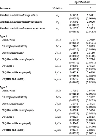
identi-fi es σε. In order to match the frequency of wage declines at job transitions shown in Panel 3 of Table 6, σε must be relatively large. However, as σε increases, σw must decrease, or else the simulated model will generate too much variation in observed wages relative to the data (Panel 1 of Table 6). In other words, when the amount of measurement error in the model is high, the amount of true variation in wage offers must be low in order to match the observed variation in wages in the NLSY97. This property of the model is demonstrated in Columns 1 and 2 of Table 2, which show the parameter estimates for a restricted version of the model that assumes that σξ = 0 along with the estimates for the unrestricted model. Finally, it is important to note that as σw decreases, the model generates lower wage gains from job search. This happens because as σw decreases, there is a lower chance that an employed worker will receive a higher outside wage offer.
Next, consider estimating a model that relaxes the restriction σξ = 0. Using only the job transition moments shown in Panel 3 of Table 6, it is impossible to separately identify σε and σξ, because a voluntary job- to- job move to a lower observed wage could be due to either mis- measurement of the wage or unobserved nonwage utility. The key to identifying the full model with nonwage utility is that during estimation, we simultaneously match moments that capture three features of the data. First, we match the amount of variation in wages (Panel 1 of Table 6). Second, we match the frequency and magnitude of wage declines at job transitions (Panel 3 of Table 6). Third, we match the amount of wage growth as refl ected in the mean wages from the
Table 2
Parameter Estimates
Specifi cations
Parameter Notation 1 2
Standard deviation of wage offers σw 0.3435 0.2691
(0.0083) (0.0044)
Standard deviation of nonwage match σξ 0.3908 0.0000
(0.0122) (—)
Standard deviation of measurement error σε 0.1672 0.2955
(0.0385) (0.0153)
Type 1
Mean wage μ(1) 1.1774 1.1689
(0.0252) (0.0191)
Unemployment utility b(1) 1.7982 1.9879
(0.0212) (0.0310)
Reservation utilitya U*(1) 1.8163 1.3150
(0.0205) (0.0116)
Pr(offer while unemployed) λu(1) 0.9198 0.3716
(0.0772) (0.0391)
Pr(layoff ) λl(1) 0.0905 0.4523
(0.0671) (0.0369)
Pr(offer while employed) λe(1) 0.4214 0.4560
(0.0663) (0.0286)
Pr(offer and layoff ) λle(1) 0.2545 0.0916
(0.0463) (0.0248)
Type 2
Mean wage μ(2) 1.7252 1.6776
(0.0151) (0.0096)
Unemployment utility b(2) 1.8370 1.7487
(0.0387) (0.0233)
Reservation utilitya U*(2) 1.8948 1.7508
(0.0196) (0.0088)
Pr(offer while unemployed) λu(2) 0.6299 0.5656
(0.0523) (0.0568)
Pr(layoff ) λl(2) 0.0529 0.0533
(0.0061) (0.0072)
Pr(offer while employed) λe(2) 0.5348 0.5349
(0.0190) (0.0190)
Pr(offer and layoff ) λle(2) 0.0214 0.0256
(0.0028) (0.0031)
Table 2 (continued)
Specifi cations
Parameter Notation 1 2
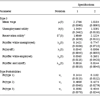
Type 3
Mean wage μ(3) 2.1766 1.8184
(0.0390) (0.0093)
Unemployment utility b(3) 1.3484 1.3291
(0.2462) (0.0118)
Reservation utilitya U*(3) 1.9869 2.1224
(0.1039) (0.0111)
Pr(offer while unemployed) λu(3) 0.1421 0.7747
(0.0106) (0.0715)
Pr(layoff ) λl(3) 0.0345 0.0306
(0.0045) (0.0055)
Pr(offer while employed) λe(3) 0.0365 0.2651
(0.0115) (0.0428)
Pr(offer and layoff ) λle(3) 0.0016 0.0144
(0.0010) (0.0045)
Type Probabilities
Pr(type 1) π1 0.1414 0.1182
(0.0113) (0.0112)
Pr(type 2) π2 0.4989 0.4274
(0.0368) (0.0279)
Pr(type 3) π3 0.3598 0.4544
(0.0370) (0.0244)
Notes: Bootstrapped standard errors in parentheses.
a. The reservation utility levels are computed by solving Equation 8 at the estimated parameters.
2. Mean transition parameters and unemployment utility fl ow
Before considering identifi cation of the mean and covariance matrix of the distribution of person- specifi c unobserved heterogeneity, we fi rst discuss how the across- type means of the parameters {b(j),
u(j),l(j),e(j),le(j)}j=1
J are identi
fi ed.
The layoff rate, λl, is identifi ed by the empirical transition rate from employment into unemployment (moment 11 in Table 6). The job offer arrival rate, λe, is identifi ed by moments that describe job- to- job transitions.31 Within the model, the probability of a job- to- job transition for a worker employed in a job with utility U is λePr(U′ > U). Taking the parametric distribution H(U) as given, λe is identifi ed by moments that
describe the frequency of job- to- job transitions, such as the empirical job- to- job tran-sition rate (moment 12).32
An important distinction between this paper and the existing literature is that we allow for three possible explanations for observed wage declines at direct job- to- job transitions. The possible explanations are measurement error in wages, involuntary job endings that occur at the same time as outside job offers, and nonwage utility. To the best of our knowledge, this is the fi rst paper to build a model that incorporates all of these explanations, and estimates the model to quantify the importance of each.33 The most straightforward of these three possible explanations from the perspective of iden-tifi cation is involuntary job endings that occur at the same time as outside job offers. The probability that this event occurs is represented in the model by the parameter λle. As discussed in Section III, we use data from the NLSY97 on the reason that jobs end to distinguish between voluntary and involuntary direct transitions between employers. If an individual reports that a job ends involuntarily, and he moves to a new job without experiencing an intervening spell of unemployment, then a simultaneous exogenous job ending and accepted outside offer has occurred. The probability that this type of transition occurs is λlePr(U′ > U*). Taking H(U) and U* as given, the fraction of direct job- to- job transitions in the data that are involuntary (moment 33) identifi es λle.
To see the importance of accounting for involuntary transitions between employers during estimation, note that within the structure of the model, a voluntary transition to a lower wage job can only be explained by measurement error or nonwage utility. In contrast, if a job exogenously ends and a new offer is received, a worker could move to a job that offers lower utility than his previous job because it is preferable to unem-ployment. More concretely, suppose that a job- paying wage w exogenously ends, and the worker simultaneously receives a new outside job offer (w′,ξ′), where w′ < w. The worker will accept a wage decrease equal to (w′ – w) instead of becoming unemployed if U(w′,ξ′) > U*. If the presence of involuntary transitions in the data was ignored dur-ing estimation, it would force the model to account for all negative wage changes at job transitions in the data with either measurement error in wages or nonwage utility.
It remains to discuss identifi cation of the utility fl ow from unemployment, b, and the arrival rate of job offers for the unemployed, λu. The reservation utility (as derived in Appendix 1) for the unemployed is defi ned by the following equation,
(8) U*=b+␦[
u−(e+le)] U*
∞
∫
(1−␦)+␦{1−H(U′)e[1−H(U′)]+l+le}
dU′,
and the transition rate out of unemployment is λuPr(U′ > U*). Note that U* is not a primitive of the model—it is determined by optimal job search behavior. During estimation, we fi x the monthly discount rate to δ = 0.998. It is clear from Equation 8 that both λu and b will impact the unemployment durations generated by the model.
32. As discussed in French and Taber (2011), non- parametric identifi cation of λe requires exclusion restric-tions in the form of observable variables that affect λe but do not affect Pr(U′ > U). In our model and with these data, there are no obvious candidates for exclusion restrictions. Unfortunately, information on rejected job offers, which would provide direct information about λe, is not available in the NLSY97.
To see how these parameters are separately identifi ed, it is useful to consider a simple thought experiment. Suppose that unemployment durations in the data are very long. There are two possible explanations for this within the context of the model. In the
fi rst explanation, both b and λu are very high, so workers remain unemployed because they receive a lot of job offers but choose to reject many offers because they place a high value on leisure. In the second explanation, both b and λu are very low, so work-ers remain unemployed because job offwork-ers are rare. The key to distinguishing between these two explanations is that they have different implications for job mobility. In the
fi rst explanation, only very good job offers are accepted by the unemployed, so initial jobs will tend to last for a long time. In the second explanation, the value of initial jobs will be lower, so workers will more frequently move to better jobs. Based on this intuition, in addition to matching features of the unemployment duration distribution during estimation (Moments 10, 18–20), we also match the mean employment dura-tion of the fi rst job in an employment cycle (Panel 1 of Table 6).
3. Identifying the distribution of unobserved heterogeneity
The fi nal group of moments shown in Panel 5 of Table 6 identifi es the distribution of person- specifi c heterogeneity in the model. In many cases, the intuition behind identifi cation of these parameters closely parallels simpler panel data models of wages and employment durations. For example, the within- person covariance in wages (Mo-ment 46) helps identify the person- specifi c component of wages, just as it would in a simpler panel data model of wages. When there is no heterogeneity in μw across people, the model generates a within- person covariance of zero between wages on employers that are separated by unemployment spells.
We have already discussed identifi cation of the mean of the unobserved heterogene-ity terms {
w(j),b(j),u(j),l(j),e(j),le(j)}j=1
J . It remains to discuss identi
fi ca-tion of the variance- covariance matrix of this distribuca-tion. Throughout this discus-sion, we take as given that the discrete distribution of unobserved heterogeneity has three points of support. As a result of this assumption, all variance- covariance terms (and means) are functions of the type- specifi c parameters and type probabilities. For example, the covariance between the mean wage offer and the layoff rate is cov(
As an example of how the covariance terms are identifi ed, consider entry (3,1) of Table 7. This entry indicates that cov(λu,μw) is identifi ed by the covariance between the unemployment duration and the wage on the fi rst job after unemployment (Mo-ment 47), and the covariance between a person’s average wage over the career and the fraction of his career spent unemployed (Moment 49). Similarly, entry (5,4) of this table shows that cov(λle,λe) is identifi ed by the covariance between the number of voluntary and involuntary job- to- job transitions that workers make over their career. The intuition is that if this empirical moment is positive, it indicates that workers who make a large number of voluntary job transitions also tend to make a large number of involuntary transitions. Within the model, these types of mobility will be positively correlated if cov(λle,λe) is positive.
In the interest of brevity, we omit further discussion of identifi cation of the covari-ance matrix because the intuition behind identifi cation of the remaining parameters closely follows the three preceding examples.
4. Heterogeneous transition parameters vs. correlation between w and ξ
Our model assumes that the wage and nonwage components of job offers are uncor-related, however, arguments can be made in favor of either positive (health insurance) or negative (risk of injury or death) correlation between w and ξ. Moments that might identify this correlation include ones that capture the relationship between wages, and voluntary job- to- job moves and job / employment durations. For example, if wage and nonwage utility offers are positively correlated then the relationship between current wages and the frequency of voluntary job- to- job moves is steeper than when they are negatively correlated. With positive correlation, a person in a high- wage job in all likelihood also has a high ξ and is less likely to move to another job voluntarily. By the converse argument, a person in a low- wage job likely also has a low ξ and job offers are likely to dominate their current job so that the worker is more likely to move to another job voluntarily.
However, because differences across individuals in expected wage offers, the value of nonemployment, and transition parameters affect these moments similarly, it is diffi cult to separately identify a correlation between wage and nonwage utility offers from across- person variation in {
w(j),b(j),u(j),l(j),e(j),le(j)}j=1
J . Indeed, we
were unable to estimate a model with both heterogeneity in transition parameters and correlation between w and ξ.
In order to understand this feature of the model, consider a simple example where there are two types of workers who differ in both mean wage offers and job offer ar-rival rates while employed.34 Suppose that type 1 workers have a low mean wage offer, μw(1), and a high job offer rate λe(1). In contrast, type 2 workers have a high μw(2), and a low λe(2). In this example, high- wage workers will tend to make fewer job- to- job transitions than low- wage workers, so wages and job- to- job mobility will be negatively correlated, just as they would be in a world where offers of w and ξ were