Published Online: May 2014
Available online at http://pphmj.com/journals/fjms.htm Volume 87, Number 1, 2014, Pages 23-35
Received: August 16, 2013; Accepted: October 8, 2013 2010 Mathematics Subject Classification: 92C55.
Keywords and phrases: stage, breast cancer, mammogram, physical parameter.
A NOVEL MODEL DETERMINATION OF BREAST
CANCER STAGE USING PHYSICAL PARAMETER
Anak Agung Ngurah Gunawan
Department of Physics University of Udayana at Bali Indonesia
e-mail: [email protected]
Abstract
This article determines the stage of breast cancer with a new method using mathematical equation models with physical parameters. To determine the stage of breast cancer, a model has been developed by the method of Tumor Node Metastasis (TNM) and Scarff-Bloom-Richardson. In this study, we have used mathematical equation models with physical parameters to determine the probability of gray-level pair at a certain distance. In a previous research, we managed to determine the histological type of breast cancer using the physical parameters. The proposed approach has been tested on 15 mammograms new patients of Dr. Soetomo Hospital, Indonesia. The results showed that the use of physical parameters was actually able to predict the stage of breast cancer with a sensitivity of 86,67% on the footage 5×5 cm and α=5%.
1. Introduction
[3], self similar fractal [4], fractal feature [5], neural network [6], Kekre’s [7], SVM classifier [8], texture resemblance marker [9], extraction [10], accurate method [11], contour description [12], bilateral asymmetry [13], orthogonal polynomials model [14], the dual tree complex [15], Gabor features [16], fuzzy clustering [17], k-means and fuzzy c-means [18], vector quantization technique [19], Kohonen SOM and LVQ network [20], entropy Sallis Q and a type II fuzzy [21], foveal method [22] and wavelet [23]. However, these methods only detect the presence of microcalcification course and not the breast cancer staging. In a previous study, we have succeeded in classifying types of breast cancer histology using physical parameters of the sensitivity of 86.36% on a 5×5 cm samples with α = 5% [24].
The paper is organized as follows: Section 2 discusses the interaction of radiation with breast cancer, Section 3 discusses the physical parameters, Section 4 discusses the logistic regression mapping function and Section 5 discusses multinomial linear regression function as the outcome of the stage type. Section 6 discusses the result and discussion and last, conclusions are discussed in Section 7.
2. Radiation Interaction with Breast Cancer
The intensity of the radiation beam on breast cancer is partly absorbed and partly transmitted. The intensity of the transmitted radiation beam of density is dependent upon the breast cancer. As the breast density becomes greater, the more the intensity of the light is absorbed or the less the intensity of the transmitted beam. The less the intensity of the transmitted light, the closer the gray-level mammogram films gets to a white color or higher pixel intensity values. Relationship intensity of the light transmitted by the density of breast cancer can be written as follows:
,
0 L
t I e
I = −μ (2.1)
3. Physical Parameters
Each level of malignancy disease has different patterns of pixel intensities. Of these patterns are probabilities pair gray-level at a certain distance. Pair of gray-level probability at any distance can be determined by lack of uniformity (entropy), sharpness structural variations (contrast), structural uniformity (angular second moment), the local homogeneity (inverse difference moment), linear dependence (correlation), authenticity properties (mean), density (deviation), lack of uniformity of the distribution of probability of occurrence gray-level pair at a certain distance (entropy of
),
diff
H structural uniformity of the distribution of probability of occurrence gray-level pair at a certain distance (angular second moment of Hdiff) and the nature of the authenticity of the pair probability distribution of gray-level events at a certain distance (mean Hdiff) as follows [24, 25]:
( )
[
(
, ,)
] [
log(
, ,)
]
,1 1
∑
=∑
= − = t q t r y y y y yy H yq yr d H yq yr d
E
Entropy (3.1)
( )
(
)
(
, ,)
, 1 1 2∑
=∑
= − = t q t r y y y y yy yq yr H yt yr d
C
Contrast (3.2)
Angular second moment
(
ASM)
[
(
, ,)
]
, 1 1 2∑
=∑
= = t q t r y y y y yy H yq yr d (3.3)
Moment differential inverse
(
MDI)
(
)
(
)
∑
=∑
= ⎥⎥ ⎦ ⎤ ⎢ ⎢ ⎣ ⎡ − + = t q t r y y y y y y r q r q y y d y y H1 1 1 2
, ,
(3.4)
for ,yr ≠ yq
Correlation
(
Corr)
(
)
(
)
(
)
(
y d)
H(
y d)
H d y H d y H d y y H y y r m q m y y y y y
y q r q r m q m r
t q t r , , , , , , 1 1 σ σ μ μ −
with
(
,)
(
, ,)
, 1∑
= = t r y yy q r
q
m y d H y y d
H (3.6)
(
,)
(
, ,)
, 1∑
= = t q y yy q r
r
m y d H y y d
H (3.7)
( )
∑
(
)
= = t q y yy yqHm yq d
M Mean 1 , , (3.8)
( )
(
,)
(
,)
, 1 1 2∑
=∑
= ⎥⎦ ⎤ ⎢⎣ ⎡ − = t q t p y yy m q
y
y
y p m p
q y H y d H y d
y D Deviation (3.9)
(
)
∑
∑
(
)
= − = = = t r q q t r y y y y y yy q r
diff i d H y y d
H
1 , , ,
,
1
(3.10)
Entropy of
(
)
(
,)
log(
,)
,1
∑
=− = it
i
i diff diff
diff EHD H i d H i d
H (3.11)
ASMof
(
,)(
)
[
(
,)
]
,1
2
∑
== it i i diff
diff i d ASMHD H i d
H (3.12)
Mean of
(
)
∑
(
)
=
= it i i diff
diff MHD iH i d
H
1
,
, (3.13)
where yq, yr, d are the gray-level pixel value of unity, the value of the second pixel gray-level and the distance between the two pixels with pixels
unity, respectively. H
(
yq, yr, d)
is a second-order histogram that describes the distribution of probability of occurrence of a pair of gray-level.4. Logistic Regression Mapping Function
Review the following probability function:
( )
Y∑
≠
j j j
i a X
X , where Y is output category, e.g., y = 0, stage 1 category,
, 1
=
y stage 2 category and so on, y = k, particular category.
This form is multinomial or multiple linear rate.
Review of the logistic function (logic) as follows [24]:
(
)
{
}
(
(
)
)
⎭ ⎬ ⎫ ⎩ ⎨ ⎧ | = − | = = | = X Y P X Y P log X Y P logic r rr 1 1
1 1
(
)
(
1)
.1 1 ln Y X Y P X Y P r r = ⎭ ⎬ ⎫ ⎩ ⎨ ⎧ | = − | = ≅ (4.1)
Further, Y :
{
Z1, Z2, Z3, Z4}
with X :{
allof entropies}
. For example, the category Y = Zk(
)
(
1)
.1 1 ln k r r Z X Y P X Y P = ⎭ ⎬ ⎫ ⎩ ⎨ ⎧ | =
− = | (4.2)
Note. Use of functional in natural logarithm related to qualitative mapping (entropy) to qualitative (stage types of breast cancer), which does not satisfy the normal Gaussian, statistically,
(
)
(
)
Zkr r e X Y P X Y P = | = − = |1 1
1
or
(
(
)
)
Zkr r e X Y P X Y
P = −
| == | − 1 1 1 to obtain:
(
1)
(
1)
,1 Zk
r
r Y X P Y X e
P = | = = | −
−
(
=1|){
1+ −Zk}
=1,r Y X e
P
(
)
{
1}
,1 1 k Z r e X Y P − + = | = (4.3)
and Pr
(
Y =1|X)
as a multinomial logistic regression of statistical model.For example
{
Y = Zk}
k=1,2, it will be found in all categories(
)
{
}
, , 3 , 1 , 2 , 1 , 1 , 1 1 3 2 1 ⎪⎭ ⎪ ⎬ ⎫ ⎪⎩ ⎪ ⎨ ⎧ = = = = detected stage Z detected stage Z detected stage Z Zk(
)
{
1}
,1 1 1 1 Z r e X Z P − + = | = (4.4)
(
)
{
1}
,1 1 2 2 Z r e X Z P − + = | = (4.5)
(
)
{
1 3}
1 1 3 Z r e X Z P − + = | = (4.6)
and because the fulfillment of all categories/stages into force,
(
1)
1,4 1
∑
k= Pr Zk = |X =(
Z1 =1|X)
+ P(
Z2 =1|X)
+ P(
Z3 =1|X)
=1,Pr r r until
(
Z1 1 X)
1 P(
Z2 1 X)
P(
Z3 1 X)
,Pr = | = − r = | − r =
(
)
{
}
{
1}
.1 1 1 1 1 3 2 1 ⎥ ⎦ ⎤ ⎢ ⎣ ⎡ + − ⎥ ⎦ ⎤ ⎢ ⎣ ⎡ + − = | = − − Z Z r e e X Z P (4.7)
5. Linear Regression Multinomial Function as an
Outcome of the Stage Type
Review the following linear regression [24]:
MeanHd10, . Bkn 1 , 0 + ⎭ ⎬ ⎫ ⎩ ⎨ ⎧ + =
∑
= n jk kj j
k
k Z B Entr
Z (5.1)
k
Z is the outcome/impact of a number of
{
Entrj}
,0
k
Z is the intersection/intersection of the axis or the initial value of outcome, .
0
k
k Z
For the tribe Bkn .MeanHd10 0, 1
, ⎭⎬+ =
⎫ ⎩
⎨ ⎧
∑
= n
j
k Bkj Entrj
∑
nk, j=1Bkj Entrj is a nuisance parameter/variable-free number{
Entrj}
the rank of 1 (one) or linear,Bkn.MeanHd10 is the correction factor by the number of outcome
{
Entrj}
.For example:
MeanHd10, .
B2n 1
,
2 2
20
2 +
⎭ ⎬ ⎫ ⎩
⎨ ⎧ +
=
∑
= n
j B j Entrj
Z
Z (5.2)
MeanHd10. .
B3n 1
,
3 3
30
3 +
⎭ ⎬ ⎫ ⎩
⎨ ⎧ +
=
∑
= n
j B jEntrj
Z
Z (5.3)
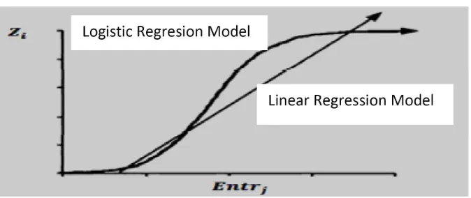
[image:7.612.130.467.334.476.2]These are illustrated in Figure 1 as follows:
Figure 1. Linear regression model and logistic regression model.
6. Results and Discussion
Figure 2. (a) Stage 1, (b) Stage 2 and (c) Stage 3. All the mammographic images are collected from the data base computer at radiodiagnostic Dr. Soetomo Hospital Indonesia, these images of mammographic labelling Kodak brand, type 6900 laser imager dryview data prints of mammographic films and it is placed in the direct view 975 CR. Images saved in bmp format and sampled with a size of 5×5cm.
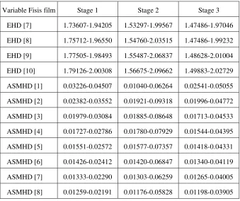
Table 1. Range value of physical parameter stage 1, stage 2 and stage 3
Variable Fisis film Stage 1 Stage 2 Stage 3
EHD [7] 1.73607-1.94205 1.53297-1.99567 1.47486-1.97046
EHD [8] 1.75712-1.96550 1.54760-2.03515 1.47486-1.99232
EHD [9] 1.77505-1.98493 1.55487-2.06837 1.48628-2.01004
EHD [10] 1.79126-2.00308 1.56675-2.09662 1.49883-2.02729
ASMHD [1] 0.03226-0.04507 0.01040-0.06264 0.02541-0.05055
ASMHD [2] 0.02382-0.03552 0.01921-0.09318 0.01996-0.04772
ASMHD [3] 0.01979-0.03084 0.01885-0.08648 0.01713-0.04533
ASMHD [4] 0.01727-0.02786 0.01780-0.07929 0.01544-0.04395
ASMHD [5] 0.01551-0.02572 0.01577-0.07357 0.01418-0.04331
ASMHD [6] 0.01426-0.02412 0.01420-0.06847 0.01340-0.04119
ASMHD [7] 0.01333-0.02290 0.01303-0.06259 0.01265-0.04005
[image:8.612.128.467.319.603.2]ASMHD [9] 0.01200-0.02098 0.01075-0.05382 0.01144-0.03791
ASMHD [10] 0.01151-0.01994 0.00998-0.04819 0.01091-0.03688
MHD [1] 9.92311-13.81787 7.03711-22.00450 8.66159-18.50292
MHD [2] 12.71444-18.85441 8.67398-23.14779 9.19399-23.10747
MHD [3] 14.71335-22.88359 10.03482-25.84119 9.71770-26.75284
MHD [4] 16.34673-26.14803 11.44139-28.45701 9.99301-29.55086
MHD [5] 17.79653-29.10036 12.41866-31.16452 10.23093-32.00988
MHD [6] 19.04117-31.69811 12.73418-34.88744 10.72127-33.90060
MHD [7] 20.13923-33.92885 12.95908-38.22411 11.04172-35.78729
MHD [8] 21.15194-35.91399 13.54083-41.38564 11.29721-37.82326
MHD [9] 22.10252-37.64858 13.72020-44.66617 11.63253-39.52103
MHD [10] 23.03941-39.22549 14.14465-47.98476 12.01704-41.35556
Mode of mathematical equations to determine the stage of breast cancer is as follows:
=
: 2
Z –893.020 + 195160.164 * ASMHD [2] – 510897.436 * ASMHD [3]
+ 533083.158 * ASMHD [4] – 269158.613 * ASMHD [5]
+ 252132.909 * ASMHD [6] – 1440.363 * ASMHD [7]
– 254114.237 * ASMHD [8] – 272372.401 * ASMHD [9]
+ 327999.228 * ASMHD [10] + 94.046 * MHD [1]
– 108.973 * MHD [2] – 1.364 * MHD [3] + 294.227 * MHD [4]
+ 17.633 * MHD [5] – 2.388 * MHD [6] – 638.598 * MHD [7]
+ 1341.563 * MHD [8] – 1927.761 * MHD [9]
=
: 3
Z –1512.837 + 148397.141 * ASMHD [2] – 348864.647 * ASMHD [3]
+ 374023.365 * ASMHD [4] + 582434.961 * ASMHD [5]
– 990621.703 * ASMHD [6] – 1598.515 * ASMHD [7]
+ 122174.826 * ASMHD [8] – 126994.804 * ASMHD [9]
+ 241438.444 * ASMHD [10] + 44.331 * MHD [1]
– 320.941 * MHD [2] – 3.389 * MHD [3] + 1645.629 * MHD [4]
– 74.639 * MHD [5] – 55.387 * MHD [6] – 4306.505 * MHD [7]
+ 5360.133 * MHD [8] – 4033.694 * MHD [9]
+ 1837.766 * MHD [10];
Probability stage 2:=1
(
1+Exp(
−Z2)
)
; Probability stage 3:=1(
1+Exp(
−Z3)
)
;Probability stage 1 := 1 – Probability stage 2 – Probability stage 3.
The optimum physical variables to classify breast cancer stage is structural uniformity of the distribution of probability of occurrence gray level pair at a distance of 2, 3, 4, 5, 6, 7, 8, 9, 10
(
angular second moment of)
diffH and the nature of the authenticity of the pair probability distribution of gray-level events at a distance of 1, 2, 3, 4, 5, 6, 7, 8, 9, 10
(
mean Hdiff)
.7. Conclusion
second moment of Hdiff
)
and the nature of the authenticity of the pair probability distribution of gray-level events at a distance of 1, 2, 3, 4, 5, 6, 7, 8, 9, 10(
mean Hdiff)
.References
[1] F. Eddaoudi and F. Regragui, Microcalcifications detection in mammographic images using texture coding, Appl. Math. Sci. 5(8) (2011), 381-393.
[2] B. Senthilkumar and G. Umamaheswari, A novel edge detection algorithm for the detection of breast cancer, European Journal of Scientific Research 53(1) (2011), 51-55.
[3] B. C. Patel and G. R. Sinha, An adaptive k-means clustering algorithm for breast image segmentation, International Journal of Computer Applications 10(4) (2010), 35-38.
[4] B. C. Patel and G. R. Sinha, Early detection of breast cancer using self similar fractal method, International Journal of Computer Applications 10(4) (2010), 39-42.
[5] D. Sankar and T. Thomas, Fractal features based on differential box counting method for the categorization of digital mammograms, International Journal of Computer Information System and Industrial Management Applications 2 (2010), 11-19.
[6] J. Dheeba and J. G. Wiselin, Detection of microcalcification clusters in mammograms using neural network, International Journal of Advanced Science and Technology 19 (2010), 13-22.
[7] H. B. Kekre, Saylee M. Gharge and Tanuja K. Sarode, Image segmentation of mammographic images using Kekre’s proportionate error technique on probability images, International Journal of Computer and Electrical Engineering 2(6) (2010), 1048-1052.
[8] F. Eddaoudi, F. Regragui, A. Mahmoudi and N. Lamouri, Masses detection using SVM classifier based on textures analysis, Applied Mathematical Sciences 5(8) (2011), 367-379.
[10] M. Vasantha, V. S. Bharathi and R. Dhamodharam, Medical image feature, extraction, selection and classification, International Journal of Engineering Science and Technology 2(6) (2010), 2071-2076.
[11] M. Rizzi, M. D. Aloia and B. Castagnolo, An accurate method to assist physicians for breast cancer detection, World Applied Sciences Journal 10(3) (2010), 348-354.
[12] P. H. Tsui, Y. Y. Liao, C. C. Chang, W. H. Kuo, K. J. Chang and C. K. Yeh, Classification of benign and malignant breast tumors by 2-d analysis based on contour description and scatterer characterization, IEEE Transactions on Medical Imaging 29(2) (2010), 513-521.
[13] S. K. Bandyopadhyay, Image processing algorithms for bilateral asymmetry detection - a survey, Journal of Global Research in Computer Science 1(3) (2010), 39-43.
[14] R. Krishnamoorthy, N. Amudhavalli and M. K. Sivakolundu, Identification of microcalcifications with orthogonal polynomials model, International Journal of Engineering Science and Technology 2(5) (2010), 1204-1210.
[15] K. Sujatha and V. C. Sumitha, Dual tree complex with modified complex ridgelets for image denoising in digital mammographic images, Proceedings of the Int. Conf. on Information Science and Applications ICISA, 2010, pp. 507-511.
[16] Y. Zheng, Breast cancer detection with Gabor features from digital mammograms, Algorithms 3 (2010), 44-62.
[17] N. K. Visalakshi, K. Thangaved and R. Parvathi, An intuitionistic fuzzy approach to distributed fuzzy clustering, International Journal of Computer Theory and Engineering 2(2) (2010), 295-302.
[18] N. Singh and A. G. Mohapatra, Breast cancer mass detection in mammograms using k-means and fuzzy c-means clustering, International Journal Computer Applications 22(2) (2011), 15-21.
[19] H. B. Kekre, Tanuja K. Sarode and Saylee M. Gharge, Tumor detection in mammography images using vector quantization technique, International Journal of Intelligent Information Technology Application 2(5) (2009), 237-242.
[20] Z. Chalabi, N. Berrached, N. Kharchouche, Y. Ghellemallah, M. Mansour and H. Mouhadjer, Classification of the medical images by the kohonen network SOM and LVQ, Journal of Applied Sciences 8(7) (2008), 1149-1158.
[22] Oh Whi-Vin, Kim KwangGi and Kim Young-Jae, Detection of microcalcifications in digital mammograms using foveal method, J. Kor. Soc. Med. Informatics 15(1) (2009), 165-172.
[23] S. Bouyahia, J. Mbainaibeye and N. Ellouze, Wavelet based microcalcifications detection in digitized mammograms, ICGST-GVIP Journal 8 (2009), 23-31.
[24] A. A. N. Gunawan, Suhariningsih, K. S. P. Triyono and B. Widodo, Determination of physical parameter model for the photo film mammographic X-ray results on the breast cancer histology classification, Int. J. Contemp. Math. Sciences 7(45) (2012), 2235-2244.