A COMPARISON OF NEIGHBOURHOOD SELECTION TECHNIQUES IN
SPATIO-TEMPORAL FORECASTING MODELS
J. Haworth a, *, T. Cheng a
a SpaceTimeLab, Dept. of Civil, Environmental and Geomatic Engineering, University College London, Gower Street, London, WC1E 6BT UK – [email protected], [email protected]
Technical Commission II
KEY WORDS: Spatio-temporal, forecasting, prediction, transportation, model selection, variable selection
ABSTRACT:
Spatio-temporal neighbourhood (STN) selection is an important part of the model building procedure in spatio-temporal forecasting. The STN can be defined as the set of observations at neighbouring locations and times that are relevant for forecasting the future values of a series at a particular location at a particular time. Correct specification of the STN can enable forecasting models to capture spatio-temporal dependence, greatly improving predictive performance. In recent years, deficiencies have been revealed in models with globally fixed STN structures, which arise from the problems of heterogeneity, nonstationarity and nonlinearity in spatio-temporal processes. Using the example of a large dataset of travel times collected on London’s road network, this study examines the effect of various STN selection methods drawn from the variable selection literature, varying from simple forward/backward subset selection to simultaneous shrinkage and selection operators. The results indicate that STN selection methods based on penalisation are effective. In particular, the maximum concave penalty (MCP) method selects parsimonious models that produce good forecasting performance.
* Corresponding author. This is useful to know for communication with the appropriate person in cases with more than one author.
1. INTRODUCTION 1.1 Space-time forecasting
Recent decades have seen an unprecedented rise in the collection, storage and analysis of data pertaining to a diverse range of processes, many of which are measured in geographic space at discrete time intervals, and can be referred to as space-time series. Often, such series describe natural or human phenomena that we would like to be able to predict, in order to manage our response. Often, physical models of these processes can be constructed. For example, series of traffic flows are often modelled using theory from fluid or gas dynamics (Hoogendoorn and Bovy, 2001). However, sometimes insufficient data are available to calibrate such models and researchers must turn to data driven techniques as an alternative. In this context, the term data driven is taken to mean those approaches that do not make any assumptions about the physical process generating the data (although they may make distributional assumptions). They attempt to model how future values of the series evolve from its current values.
Broadly, data driven approaches to space-time forecasting can be separated into two categories: 1) parametric, and 2) non-parametric. Parametric models assume that the data follow a particular parametric distribution, and that the future values of the process can be modelled as a (usually linear) combination of its past values. Examples of parametric space-time forecasting models include the space-time autoregressive integrated moving average (STARIMA) modelling framework ((Pfeifer and Deutsch, 1980); (Kamarianakis and Prastacos, 2005), state-space models ((Stathopoulos and Karlaftis, 2003), Bayesian networks (Sun et al., 2005) to name but a few.
Nonparametric approaches typically don’t make explicit distributional assumptions and try to learn the relevant characteristics of the data directly through exposure to examples. The most commonly used nonparametric method is the artificial neural network (ANN), which has been used widely in traffic forecasting (Van Lint et al., 2005), (Vlahogianni et al., 2005). Other commonly used methods include various forms of nonparametric regression (Smith et al., 2002); (Clark, 2003) and kernel methods (Chun-Hsin Wu et al., 2004); (Castro-Neto et al., 2009)). Each approach has its strengths and weaknesses, and (Karlaftis and Vlahogianni, 2011) provide a good overview, but the task is the same: to create a model that can effectively describe the spatio-temporal evolution of the process.
Crucial to building an effective space-time forecasting model is determining the most relevant information to input to the model. This is a case of defining the spatio-temporal neighbourhood (STN), which is the neighbourhood of spatial and temporal information that is required to forecast some quantity at a given location and time. From the perspective of statistical modelling, this is a problem of variable selection. Variable selection is an active research area, particularly in the machine learning community. The method that has been traditionally applied to problems with few variables is subset selection (forward or backward). However, subset selection is computationally infeasible in high dimensional data (Fan and Lv, 2010).
In spatio-temporal modelling, researchers use autocorrelation functions to quantify the relationship between measurement locations, and use the results to calibrate statistical models (Cheng et al., 2012); (Cheng et al., 2014). Typically it is assumed that spatio-temporal autocorrelation decays with distance in space and time, and becomes negligible at a certain The International Archives of the Photogrammetry, Remote Sensing and Spatial Information Sciences, Volume XL-2, 2014
spatial and temporal separation. Most space-time models, such as space-time Kriging models, assume that this relationship is stationary and isotropic (Kyriakidis and Journel, 1999).
Sometimes, however, the precise form of the spatio-temporal relationship between measurement locations is unclear, either due to the nonstationarity and heterogeneity of the space-time process or uncertainty in the data collection process. In this case, it is necessary to take a different approach. One approach is to use variable selection methods to select the independent variables based on the strength of statistical relationship with the dependent variable. This approach has been taken recently in the context of spatial modelling (Wheeler, 2009), and spatio-temporal modelling.
(Gao et al., 2011) used the graphical least absolute shrinkage and selection operator (GLASSO) to define the spatio-temporal neighbourhood in the context of traffic flow forecasting. The method estimates a sparse graph by shrinking the elements of the inverse covariance matrix towards zero. Nonzero elements can be viewed as conditionally independent and remain in the model. In a related approach, (Kamarianakis et al., 2012) used the least absolute shrinkage and selection operator (LASSO) to estimate a time varying threshold regression model, tailored to different traffic states. The aforementioned approaches do not make assumptions about the nature of the spatio-temporal relationship between locations, instead learning it from the data.
In this paper, four methods of STN selection, drawn from the variable selection literature, are compared in the context of forecasting travel times on London’s roads. The structure of the paper is as follows. In section 2, the four STN selection methods are described, which are: 1) Forward backward selection; 2) LASSO; 3) smoothly clipped absolute deviation (SCAD); and 4) maximum concave penalty (MCP). Following this, in section 3, the case study data are introduced. In section 4, an exploratory spatio-temporal data analysis is carried out to motivate the use of variable selection. In section 5, the details of the implementation are described. The results are presented in section 5, before some conclusions and directions for future research are offered in section 6.
2. METHODOLOGY 2.1 STN Selection algorithms
In this section, the four variable selection methods used for STN selection are introduced.
2.2 Forward/backward selection
Forward and backward selection are traditional methods for variable selection in regression models. They involve adding or removing variables from a larger set one by one, testing the effect on some evaluation criterion, such as the adjusted R-square, Akaike information criterion (AIC) or Bayesian information criterion (BIC). In this case, the AIC is used, and both forward and backward selection are tested. The AIC and BIC are described in, for example, (Fan and Lv, 2010).
2.3 Lasso
The least absolute shrinkage and selection operator (LASSO) is a simultaneous variable selection and regression technique that minimizes the sum of squared errors (SSE) subject to the sum of the absolute values of the regression coefficients being less than
a constant (Tibshirani, 1996). This constraint causes some of the coefficients of the model to shrink to zero, thus eliminating them from the model. It is similar in motivation to the well-known ridge regression, which places a constraint on the squared values of the coefficients, but doesn’t shrink any to zero. LASSO minimises the SSE:
(1)
Where is a penalty function and is a tuning parameter, and are the observation of the independent variable and the independent variables, respectively, , , is the number of observations, is the number of variables, is the parameter and is the absolute value of . Using the least angle regression (LAR) approach to fit the LASSO model enables the full set of solutions (the LASSO path) to be computed efficiently, making LASSO very fast computationally (Efron et al., 2004). By shrinking coefficients to zero, LASSO adds interpretability to the coefficients of the model, which is particularly important in high dimensional data. In the spatio-temporal setting, it can help to reveal spatio-temporal dependency relationships.
2.4 SCAD
Smoothly clipped absolute deviation (SCAD) is another approach to simultaneous variable selection and regression with the same motivation as LASSO (Fan and Li, 2001). Like LASSO, SCAD minimises the SSE subject to a constraint on the absolute values of the coefficients, minimizing Equation 2:
(2)
Where:
(3)
Differentiating with respect to :
(4)
The notation is the same as Equation 1, where is an additional parameter. The difference between LASSO and SCAD is that SCAD produces parameter estimates that are as efficient as if the true model were known, which is referred to as the oracle property (Wang et al., 2007). Unlike the LASSO, it is not possible to compute the full path of all possible values in the same time as the OLS estimate, so the parameters must be tuned.
2.5 MCP
The third method is the maximum concave penalty (MCP), which is also a simultaneous model selection and regression technique (Zhang, 2010). MCP provides convexity of the penalised cost according to thresholds for variable selection and unbiasedness. It therefore avoids some of the bias associated with the LASSO technique. Like LASSO, the solutions for the MCP can be calculated efficiently for all possible values of the penalty, giving a path of solutions from the non-penalized least squares solution to infinite penalty. MCP again minimises Equation 2, where:
(5)
Differentiating with respect to :
(6)
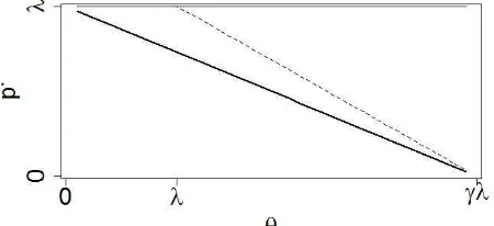
Figure 1 shows the shape of the penalty functions of each of the three algorithms (reproduced from (Breheny and Huang, 2011). Both the SCAD and the MCP gradually decrease the penalty as the size of the coefficient increases towards , at which point no penalty is applied. The effect of this is that small coefficients are shrunk towards zero while large coefficients are not shrunk.
Figure 1. Shape of first derivate of the penalty functions ( for the LASSO (horizontal line, top), SCAD (dashed line) and
MCP.
3. DATA DESCRIPTION
The data are link based unit travel times (UTT, seconds/metre), collected using automatic number plate recognition (ANPR) technology, as part of Transport for London’s (TfL’s) London Congestion Analysis Project (LCAP). ANPR cameras are installed on the road network, usually at intersections, and read the number plates of vehicles as they pass. The cameras operate in pairs ; at time a vehicle passes camera and the time is recorded. It then traverses the link and passes camera at time , and the time is recorded again. The individual travel time (ITT) is calculated as . ITTs are aggregated at 5 minute intervals to give the UTT observations presented here.
This study focuses on those links located within London’s Congestion Charging Zone (CCZ), which is shown in Figure 2.
In total, there are 80 links for which good quality data (deemed as a missing rate <75%) are available within the CCZ.
Figure 2. The location of the test links within the CCZ
Some characteristics of the study area should be noted that warrant the use of variable selection:
1. The spatial coverage of the network is sparse, and not fully coincident with the physical road network.
2. Links can overlap, meaning that some links carry the same vehicles at the same time along part of their length.
3. The level of missing data is often high, meaning that spatial information is required in forecasts.
4. EXPLORATORY SPATIO-TEMPORAL DATA ANALSYSIS
In order to ascertain what type of STN is likely to be required in a space-time model, it is advisable to carry out exploratory spatio-temporal data analysis (ESTDA). ESTDA involves examining the spatio-temporal characteristics of the data through data analysis and visualisation techniques. In this case, we use the cross-correlation function (CCF) to examine the pair-wise cross correlations (CCs) between each of the links in the test network. The CCF is an extension of the Pearson coefficient to bivariate time series. Given two time series and
, the CCF at lag is given as:
(7)
Where and are the standard deviations, , and and the means, of series and respectively. The CCF is a global measure of correlation that measures the average relationship between two variables and therefore cannot provide any information on the time varying relationship. The aim of the CCF analysis is twofold: 1) to determine whether significant CC exists between UTTs observed at different locations, and; 2) to determine whether the level of correlation decays smoothly with distance. The second point is important in determining which model to use. Prior to the analysis, a first order difference is applied to the data to ensure temporal stationarity. This avoids time of day effects causing spurious correlations to be observed.
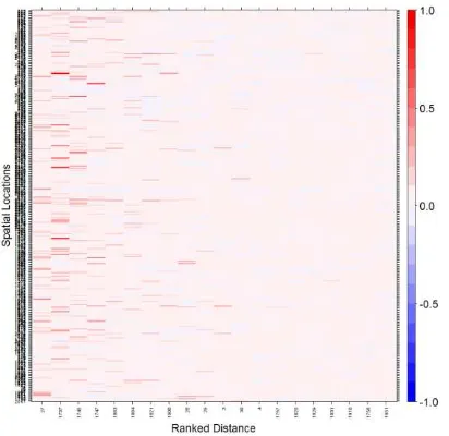
Figure 3. Cross-correlations ranked by network distance from the midpoint of each link.
Figure 3 shows the CCF between each link and its 100 nearest neighbours, ranked by network distance from midpoint to midpoint. A general distance decay relationship can be observed, although the decay is not linear. This is due to the sparse coverage of the sensor network and the difficulty in defining a proximity measure between sensor locations. Superficially, this result indicates heterogeneity in the spatial relationship between links and their neighbours, implying that a global model describing the relationship between locations will be insufficient (e.g. a STARIMA model) and a spatially local approach is required. Additionally, it can be assumed that the nearest neighbours in terms of network distance are not necessarily the best predictors. This motivates the use of the variable selection methods that are outlined here.
5. IMPLEMENTATION 5.1 STN Selection
The neighbourhood selection techniques are tested under the assumption that data from the link to be forecast are missing. There are two reasons for this: 1) Due to the spatial sparsity of the network, the level of temporal autocorrelation present in the data is much higher than the level of spatial autocorrelation, meaning that univariate techniques tend to perform very well. It should be noted that this would not necessarily be the case in other applications; 2) Removing the effect of serially autocorrelated data from the forecasts enables the spatio-temporal contribution of the model to be examined more clearly. For each method, a maximum spatial and temporal extent for the STN is defined, from which the optimal STN is selected. In this case, the maximum spatial order is set to , and the maximum temporal order is set to . This means that, for each link, the model will be comprised of a maximum of variables. For the purposes of this study, the assumption is made that spatio-temporal autocorrelation will be negligible outside this range.
5.2 Model Training
To train the models, the data are divided into a training set and a testing set. The training set comprises the first 80 days (14400 points) of the data, and the testing set comprises the next 37 days (6660 points). As the LASSO, MCP and SCAD models
require the training of hyperparameters, fold cross-validation is used within the training set. -fold cross validation involves dividing the training data into subsets, or folds. Each fold is left out of the model in turn and is forecast using the remaining folds. The selected model is the one that minimises an error criterion across the folds. In this case the root mean squared error (RMSE) is used, which is defined as follows:
(8)
Where and are the observed and forecast values, respectively. The selected model is the one that produces the lowest RMSE.
6. RESULTS
Table 1 shows the number and percentage of links for which each method performed best. It can be seen that the regularised models perform better in almost all cases. Of the LASSO, MCP and SCAD, the LASSO performs best, with the lowest RMSE in 45% of cases. However, the SCAD and MCP also perform well. It can be surmised from this result that the performance of the three regularised methods is comparable, and the choice between the three can be taken qualitatively.
Table 1. Count and percentage of best performing models
Model LM F/B LASSO MCP SCAD
Count 1 0 36 16 27
% 1.25 0 45 20 33.75
The LASSO, as well as exhibiting the best performance, has the clear advantage in terms of ease of implementation because LARS can be used. However, in space-time analysis, interpretability of the model parameters is also a concern. By examining the parameters of the model, one can begin to investigate the nature of the dependency relationships being modelled. In general, having fewer parameters makes the model more interpretable. Table 2 shows the average number of nonzero coefficients of each of the regularised models.
Table 2. Average number of nonzero coefficients of the regularized models
Model LASSO MCP SCAD
Avg. coefs. >0 27.9 15.4 19.6
The MCP generally results in a more parsimonious model with fewer coefficients. The LASSO tends to leave significantly more nonzero coefficients, while SCAD is somewhere in between. SCAD and the MCP choose fewer nonzero coefficients because they place lower penalty on larger coefficients, which are shrunk at a lower rate than smaller coefficients. This means that the dominant variables retain more of their influence on the model. Aside from the principle of parsimony, the selection of fewer variables adds explanatory power to the models.
7. CONCLUSIONS
In this study, a number of STN selection methods have been evaluated in the context of forecasting travel times under the assumption of missing data. In agreement with previous studies, it has been found that regularised methods perform well, due to their ability to simultaneously shrink and select variables. Of the three methods tested here, the LASSO exhibits the best performance, supporting the findings of (Kamarianakis et al., 2012), but is generally comparable with the MCP and SCAD. Due to the increased model parsimony offered by the MCP method, it is recommended that MCP is used where explanatory power is required in the model. The advantage of this would become more marked when dealing with data of much higher dimensionality, for example, if additional variables such as weather, traffic flows from loop detectors, and multimodal traffic information were incorporated. In future work, the MCP will be applied to time varying model structures.
It should be noted that the models tested here do not explicitly account for spatio-temporal autocorrelation in the way that models such as STARIMA do. The heterogeneity of the data in question renders the global structure of the STARIMA model insufficient in this case, but there has been research recently into regularised models that can deal with spatial heterogeneity. For example, the geographically weighted lasso (GWL) model of (Wheeler, 2009) places an penalty on the coefficients of a geographically weighted regression (GWR) model. GWR has recently been extended to the space-time domain (see, for example, (Huang et al., 2010)(Wu et al., 2014)), but the problem of variable selection has not yet been addressed in this context.
Finally, the analysis presented here focusses on the class of linear regression models. However, variable selection is also of major concern in the class of nonlinear machine learning algorithms that have been frequently applied to traffic forecasting. In previous research, the authors investigated the use of the GLASSO for time varying STN selection (Haworth
This paper is part of the EPSRC funded STANDARD (Spatio-Temporal Analysis of Network Data and Route Dynamics) project (EP/G023212/1). The author’s would like to acknowledge the support of the Road Network Perfomance & Research (RNPR) team.
REFERENCES
Breheny, P., Huang, J., 2011. Coordinate descent algorithms for nonconvex penalized regression, with applications to biological feature selection. Ann. Appl. Stat. 5, 232–253. doi:10.1214/10-AOAS388
Castro-Neto, M., Jeong, Y.S., Jeong, M.K., Han, L.D., 2009. Online-SVR for short-term traffic flow prediction under typical and atypical traffic conditions. Expert Syst. Appl. 36, 6164– 2014. A Dynamic Spatial Weight Matrix and Localized Space– Time Autoregressive Integrated Moving Average for Network Modeling. Geogr. Anal. 46, 75–97. doi:10.1111/gean.12026 Chun-Hsin Wu, Jan-Ming Ho, Lee, D.T., 2004. Travel-time prediction with support vector regression. Intell. Transp. Syst. IEEE Trans. On 5, 276–281. doi:10.1109/TITS.2004.837813 Clark, S., 2003. Traffic Prediction Using Multivariate Nonparametric Regression. J. Transp. Eng. 129, 161–168. doi:10.1061/(ASCE)0733-947X(2003)129:2(161)
Efron, B., Hastie, T., Johnstone, I., Tibshirani, R., 2004. Least angle regression. Ann. Stat. 32, 407–499.
Fan, J., Li, R., 2001. Variable selection via nonconcave
Gao, Y., Sun, S., Shi, D., 2011. Network-scale traffic modeling and forecasting with graphical lasso. Adv. Neural Networks– ISNN 2011 151–158.
Haworth, J., Cheng, T., 2014. Graphical LASSO for local spatio-temporal neighbourhood selection, in: Proceedings the GIS Research UK 22nd Annual Conference. Presented at the GISRUK 2014, University of Glasgow, Glasgow, Scotland, pp. 425–433.
Hoogendoorn, S.P., Bovy, P.H.L., 2001. State-of-the-art of vehicular traffic flow modelling. Proc. Inst. Mech. Eng. Part J.
Syst. Control Eng. 215, 283–303.
doi:10.1177/095965180121500402
Huang, B., Wu, B., Barry, M., 2010. Geographically and temporally weighted regression for modeling spatio-temporal variation in house prices. Int. J. Geogr. Inf. Sci. 24, 383–401. doi:10.1080/13658810802672469
Kamarianakis, Y., Prastacos, P., 2005. Space-time modeling of traffic flow. Comput. Geosci. 31, 119–133.
Kamarianakis, Y., Shen, W., Wynter, L., 2012. Real-time road traffic forecasting using regime-switching space-time models and adaptive LASSO. Appl. Stoch. Models Bus. Ind. 28, 297– 315. doi:10.1002/asmb.1937
Karlaftis, M.G., Vlahogianni, E.I., 2011. Statistical methods versus neural networks in transportation research: Differences, similarities and some insights. Transp. Res. Part C Emerg. Technol. 19, 387–399. doi:10.1016/j.trc.2010.10.004
Kyriakidis, P.C., Journel, A.G., 1999. Geostatistical space–time models: a review. Math. Geol. 31, 651–684.
Pfeifer, P.E., Deutsch, S.J., 1980. A Three-Stage Iterative Procedure for Space-Time Modelling. TECHNOMETRICS 22, 35–47.
Smith, B.L., Williams, B.M., Keith Oswald, R., 2002. Comparison of parametric and nonparametric models for traffic flow forecasting. Transp. Res. Part C Emerg. Technol. 10, 303– 321. doi:10.1016/S0968-090X(02)00009-8
Stathopoulos, A., Karlaftis, M.G., 2003. A multivariate state space approach for urban traffic flow modeling and prediction. Transp. Res. Part C Emerg. Technol. 11, 121–135. doi:10.1016/S0968-090X(03)00004-4
Sun, S., Zhang, C., Zhang, Y., 2005. Traffic flow forecasting using a spatio-temporal bayesian network predictor. Artif. Neural Netw. Form. Models Their Appl.-ICANN 2005 273– 278.
Tibshirani, R., 1996. Regression Shrinkage and Selection via the Lasso. J. R. Stat. Soc. Ser. B Methodol. 58, 267–288. doi:10.2307/2346178
Van Lint, J.W.C., Hoogendoorn, S.P., Van Zuylen, H.J., 2005. Accurate freeway travel time prediction with state-space neural The International Archives of the Photogrammetry, Remote Sensing and Spatial Information Sciences, Volume XL-2, 2014
networks under missing data. Transp. Res. Part C Emerg. Technol. 13, 347–369.
Vlahogianni, E.I., Karlaftis, M.G., Golias, J.C., 2005. Optimized and meta-optimized neural networks for short-term traffic flow prediction: A genetic approach. Transp. Res. Part C Emerg. Technol. 13, 211–234. doi:10.1016/j.trc.2005.04.007 Wang, H., Li, R., Tsai, C.-L., 2007. Tuning parameter selectors for the smoothly clipped absolute deviation method. Biometrika 94, 553–568. doi:10.1093/biomet/asm053
Wheeler, D.C., 2009. Simultaneous coefficient penalization and model selection in geographically weighted regression: the geographically weighted lasso. Environ. Plan. A 41, 722 – 742. doi:10.1068/a40256
Wu, B., Li, R., Huang, B., 2014. A geographically and temporally weighted autoregressive model with application to housing prices. Int. J. Geogr. Inf. Sci. 28, 1186–1204. doi:10.1080/13658816.2013.878463
Zhang, C.-H., 2010. Nearly unbiased variable selection under minimax concave penalty. Ann. Stat. 38, 894–942. doi:10.1214/09-AOS729
8.