Slide PSI 106 Materi Kuliah Statistik

McGraw-Hill/Irwin Copyright © 2010 by The McGraw-Hill Companies, Inc. All rights reserved.

Dot Plots



Mengelompokkan data sesederhana

mungkin



identitas data secara

individual tetap ada



Data ditampilkan dalam bentuk titik

sepanjang garis horisontal sesuai

nilainya

4-3

Dot Plots - Contoh

Distribusi Frekuensi



Distribusi Frekuensi diguanakan untuk

mengorganisasikan data ke dalam bentuk

yang memiliki arti



Keuntungan Distribusi Frekuensi: gambaran

visual tentang bentuk penyebaran data



Kerugian Distribusi Frekuensi:

(1)

Hilangnya identitas asli setiap nilai

(2)

Sulit melihat penyebaran nilai tiap kelas

4-5

Stem-and-Leaf



Tiap nilai dibagi dua. Digit utama menjadi

STEM dan digit sisanya menjadi LEAF. Stem

dituliskan secara vertikal, Leaf dituliskan

secara horisontal

4-7



Cara alternatif (selain standar deviasi) untuk

menggambarkan penyebaran data adalah

dengan menentukan LOKASI NILAI yang

membagi data menjadi beberapa bagian yang

setara



QUARTILES =

KUARTIL

(DIBAGI 4)



DECILES =

DESIL

(DIBAGI 10)



PERCENTILES =

PERSENTIL

( DIBAGI 100)

4-9



L

p

=

persentil yang dicari (misalnya Persentil 33



L

₃₃₎ 

n =

jumlah data



Median =

L

₅₀



Syarat: Median



data diurutkan

Percentiles - Example

Listed below are the commissions earned

last month by a sample of 15 brokers at

Salomon Smith Barney’s Oakland,

California, office.

$2,038 $1,758 $1,721 $1,637 $2,097 $2,047 $2,205 $1,787 $2,287 $1,940 $2,311 $2,054 $2,406 $1,471 $1,460

4-11

Percentiles

–

Example (cont.)

Step 1: Organize the data from lowest to

largest value

$1,460

$1,471

$1,637

$1,721

$1,758

$1,787

$1,940

$2,038

$2,047

$2,054

$2,097

$2,205

Percentiles

–

Example (cont.)

4-13

Boxplot Example

Step1: Create an appropriate scale along the horizontal axis.

Step 2: Draw a box that starts at Q1 (15 minutes) and ends at Q3 (22

minutes). Inside the box we place a vertical line to represent the median (18 minutes).

4-15

Skewness



In Chapter 3, measures of central location (the

mean, median, and mode) for a set of observations

and measures of data dispersion (e.g. range and the

standard deviation) were introduced



Another characteristic of a set of data is the shape.



There are four shapes commonly observed:

–

symmetric,

–

positively skewed,

–

negatively skewed,

4-17

Skewness - Formulas for Computing

Koefisien skewness berkisar antara -3 sampai 3.

–

Nilai berkisar -3



skewness negatif

–

Nilai 1.63



skewness cukup positif

Skewness

–

An Example



Following are the earnings per share for a sample of

15 software companies for the year 2007. The

earnings per share are arranged from smallest to

largest.



Compute the mean, median, and standard deviation.

Find the coefficient of skewness using Pearson’s

estimate.

4-19

Skewness

–

An Example Using

Pearson’s Coefficient

4-21

Describing Relationship between Two

Variables



When we study the relationship

between two variables we refer to the

data as bivariate.



One graphical technique we use to

show the relationship between

variables is called a scatter diagram.

Describing Relationship between Two

4-23

In Chapter 2 we presented data from AutoUSA. In this case the information concerned the prices of 80 vehicles sold last month at the Whitner Autoplex lot in

Raytown, Missouri. The data shown include the selling price of the vehicle as well as the age of the purchaser.

Is there a relationship between the selling price of a vehicle and the age of the purchaser?

Would it be reasonable to conclude that the more expensive vehicles are purchased by older buyers?

Describing Relationship between Two

Describing Relationship between Two

4-25

Contingency Tables



A scatter diagram requires that both of the

variables be at least

interval scale

.



What if we wish to study the relationship

between two variables when one or both are

Contingency Tables

A contingency table is a cross-tabulation that

simultaneously summarizes two variables of interest.

Examples:

1.

Students at a university are classified by gender and class rank.

2.

A product is classified as acceptable or unacceptable and by the

shift (day, afternoon, or night) on which it is manufactured.

3.

A voter in a school bond referendum is classified as to party

4-27

Contingency Tables

–

An Example

A manufacturer of preassembled windows produced 50 windows yesterday. This morning the quality assurance inspector reviewed each window for all quality aspects. Each was classified as acceptable or unacceptable and by the shift on which it was produced. Thus we reported two variables on a single item. The two variables are shift and quality. The results are reported in the following table.

Using the contingency table able, the quality of the three shifts can be compared. For example:

1. On the day shift, 3 out of 20 windows or 15 percent are defective. 2. On the afternoon shift, 2 of 15 or 13 percent are defective and 3. On the night shift 1 out of 15 or 7 percent are defective.

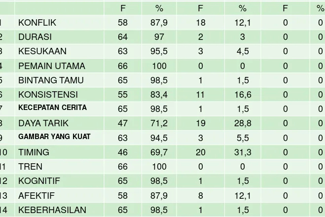
URAIAN TINGGI SEDANG RENDAH

F % F % F %

1 KONFLIK 58 87,9 18 12,1 0 0

2 DURASI 64 97 2 3 0 0

3 KESUKAAN 63 95,5 3 4,5 0 0

4 PEMAIN UTAMA 66 100 0 0 0 0

5 BINTANG TAMU 65 98,5 1 1,5 0 0

6 KONSISTENSI 55 83,4 11 16,6 0 0

7 KECEPATAN CERITA _{65 98,5 1 1,5 0 0}

8 DAYA TARIK 47 71,2 19 28,8 0 0

9 GAMBAR YANG KUAT _{63 94,5 3 5,5 0 0}

10 TIMING 46 69,7 20 31,3 0 0

11 TREN 66 100 0 0 0 0

12 KOGNITIF 65 98,5 1 1,5 0 0

4-29

DATA

KARAKTERISTIK RESPONDEN

VARIABEL KATEGORI JUMLAH PERSEN

JENIS KELAMIN PRIA 31 47

WANITA 35 53

USIA 12 - 19 3 4,5

20-29 18 27,3

30-39 20 30,3

40-49 15 22,7

50-59 9 13,6

>60 1 1,5

PEKERJAAN PNS 8 12,1

KARYAWAN 18 27,3

IRT 21 31,8

PELAJAR 6 9,1

WIRASWASTA 4 6,1

PEDAGANG 2 3

BURUH 3 4,5