HYPERSPECTRAL DATA CLASSIFICATION USING FACTOR GRAPHS
Aliaksei Makarau, Rupert M ¨uller, Gintautas Palubinskas, and Peter Reinartz
German Aerospace Center (DLR)
German Remote Sensing Data Center (DFD) bzw. Remote Sensing Technology Institute (IMF) 82234 Oberpfaffenhofen, Germany
{aliaksei.makarau, rupert.mueller, gintautas.palubinskas, peter.reinartz}@dlr.de
Commission VII/3
KEY WORDS: Hyper spectral, Classification, Training, Reference Data
ABSTRACT:
Accurate classification of hyperspectral data is still a competitive task and new classification methods are developed to achieve desired tasks of hyperspectral data use. The objective of this paper is to develop a new method for hyperspectral data classification ensuring the classification model properties like transferability, generalization, probabilistic interpretation, etc. While factor graphs (undirected graphical models) are unfortunately not widely employed in remote sensing tasks, these models possess important properties such as representation of complex systems to model estimation/decision making tasks.
In this paper we present a new method for hyperspectral data classification using factor graphs. Factor graph (a bipartite graph consisting of variables and factor vertices) allows factorization of a more complex function leading to definition of variables (employed to store input data), latent variables (allow to bridge abstract class to data), and factors (defining prior probabilities for spectral features and abstract classes; input data mapping to spectral features mixture and further bridging of the mixture to an abstract class). Latent variables play an important role by defining two-level mapping of the input spectral features to a class. Configuration (learning) on training data of the model allows calculating a parameter set for the model to bridge the input data to a class.
The classification algorithm is as follows. Spectral bands are separately pre-processed (unsupervised clustering is used) to be defined on a finite domain (alphabet) leading to a representation of the data on multinomial distribution. The represented hyperspectral data is used as input evidence (evidence vector is selected pixelwise) in a configured factor graph and an inference is run resulting in the posterior probability. Variational inference (Mean field) allows to obtain plausible results with a low calculation time. Calculating the posterior probability for each class and comparison of the probabilities leads to classification. Since the factor graphs operate on input data represented on an alphabet (the represented data transferred into multinomial distribution) the number of training samples can be relatively low.
Classification assessment on Salinas hyperspectral data benchmark allowed to obtain a competitive accuracy of classification. Employ-ment of training data consisting of 20 randomly selected points for a class allowed to obtain the overall classification accuracy equal to 85.32% and Kappa equal to 0.8358. Representation of input data on a finite domain discards the curse of dimensionality problem allowing to use large hyperspectral data with a moderately high number of bands.
1 INTRODUCTION
Development of new methods for single/multisensory data clas-sification leads to an improvement of the data clasclas-sification and a more precise identification of land-cover classes. Nevertheless, requirements on the methods such as transferability, integration into complex systems, or augmenting ability motivate an employ-ment of probabilistic graphical models [Bishop, 2006]. Applica-tion of probabilistic graphical models becomes more and more popular and efficient solution for image annotation, classification, for definition of semantic link between data and a high level la-bels [Lienou et al., 2010], [Bratasanu et al., 2011], [Wang et al., 2009].
Factor graphs (FG) were proposed in 1997 [Kschischang et al., 2001] and since then the application of FGs for signal/image processing and recognition is gradually emerging. B. Frey et al. [Frey and Jojic, 2005] performed a work on a comparison of learning and inference methods for probabilistic graphical mod-els (Bayesian networks, Markov random fields, factor graphs). Factor graph is a convenient tool to define complex systems for data processing/interpretation, to expand the systems, allow to model complex interactions among a system parts (e.g. map fea-tures/properties from low to high level), to perform approximate inference on data, or use non full data for plausible decision mak-ing. Nevertheless, application of factor graphs as a more general
graphical model type is not so wide for remotely sensed data in-terpretation.
In this paper a new approach for hyperspectral imagery super-vised classification using factor graph is proposed. The structure of the factor graph is defined in order to define prior probabilities for input data, to map the input data to a latent variable (a mixture of the input features) and bridge the mixture to a semantic class. A configuration of the factor graph on training data allows to es-timate the parameter set of the graph (probabilistic functions in the factors) and an employment of a fast inference method (Mean field [Frey and Jojic, 2005]) allows to obtain a competitive accu-racy of the hyperspectral data classification.
2 FACTOR GRAPH MODEL FOR CLASSIFICATION
Factor graph (undirected probabilistic model) is a more general graphical model than a Bayesian network or a Markov random field. An FG possesses properties of Bayesian network and Markov random field and allows to describe complex relationships among parts of a modeled system. A factor graph is a bipartite graph containing two types of nodes: variable nodes (xi, i= 1..n) and
function nodes (factors) (fj(x1, x2, . . . , xn), j = 1..m), where
a variable nodexitakes value on a finite domain (alphabetAi)
[Kschischang et al., 2001]. Figure 1 presents an example of
International Archives of the Photogrammetry, Remote Sensing and Spatial Information Sciences, Volume XXXIX-B7, 2012 XXII ISPRS Congress, 25 August – 01 September 2012, Melbourne, Australia
a factor graph with three variablesx1, x2, x3and two function
nodesf1andf2with factorization:g(x1, x2, x3) =f1(x1, x2)∗
f2(x2, x3).
Figure 1: An illustrative example of simple factor graph with three variablesx1, x2, x3and two function nodesf1(x1, x2)and
f2(x2, x3).
The task of classification consists of determining the probability of a particular hypothesis given some observed evidence. This is solved by calculation of marginal probability of a latent variable, or by calculating of the maximum likelihood probability (max-imum likelihood on the configured factor graph given the evi-dence). The likelihood of the evidence (the features vector) can be written as follows:
wherexis the input evidence;skis the class;ckis the features mixture (a latent variable);Kis the number of classes;Nis the number of features in the input evidence vector. Here, the feature is assumed to be a spectral band value.
The following factor graph structure can be defined for formula (1):
Figure 2: Factor graph model (independent model; a mixture la-tent variable is employed) for hyperspectral data classification
The factor graph is described as:
g(x1, x2, . . . , xN, ck, ss) =
wherexnis then-th input feature;ckis the features mixture (a
latent variable) for thek-th class; sk is thek-th class number;
z1, . . . , zN,zsare normalizing factors in the graph model [Frey
and Jojic, 2005] (define prior probabilities);f1, . . . , fN are the
factors mapping the input features to the feature mixture;fc−sis the factor bridging the latent variable to the semantic classsk.
The structure of a factor graph defines a dependency of class vari-able node on input features. Use of training data allows to calcu-late a configuration (parameter setθ(k)) for a factor graph for each classk.
A configured factor graph with the configurationθ(k)is expected to have a maximum likelihood probability (a low energy state) on
the evidence which most likely (similar) to the employed training data. Expectation maximization method with gradient ascent op-timizer are employed for learning the graph configuration. Mean field inference method [Frey and Jojic, 2005] is employed for the inference. Comparison of the classes probability maps (maxi-mum principle) allows to produce label map.
2.1 Employed data
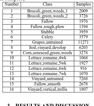
Salinas hyperspectral data benchmark (AVIRIS sensor over Sali-nas Valley, California; 3.7 m pixel size) was selected for classi-fication accuracy evaluation. The data cube size is 512 lines by 217 samples, 224 bands. 19 water absorption bands were dis-carded (bands [108-112] and [154-167]) This image is available as at-sensor radiance data. Ground truth classes and the number of samples are given in Table 1.
Minimum noise fraction (MNF) [Green et al., 1988, Boardman and Kruse, 194] was employed to reduce the number of input features, reduce computational time, and separate noise from the data. The MNF consists of two Principal Components (PC) trans-formations. The first PC transformation decorrelates and rescales noise in the data, the second PC transformation performed on the noise-cleared data.
Since factor graphs are discrete graphical models, the feature is to be represented on a predefined finite domain (alphabet). The fi-nite domain refers to the unique values (or a list of values) the fea-ture can have. Here we use a finite domain consisting of natural numbers. To represent an input feature on the finite domain, the feature is proposed to be processed separately by an unsupervised clustering. A cluster’s number is assumed as the value from the defined domain.k-means procedure is employed and the number of clusters for feature representation on finite set was equal to 100 (used for representation of all features). In an additional experi-ment, the features before representation are processed by median filtering.
20 points were randomly selected for each class in order to con-figure the factor graph. Expectation maximization with a gradient ascent method were employed for the factor graph configuration.
Table 1: Salinas hyperspectral benchmark classes (available ground truth samples)
Number Class Samples 1 Brocoli green weeds 1 2009 2 Brocoli green weeds 2 3726 3 Fallow 1976 9 Corn senesced green weeds 3278 10 Lettuce romaine 4wk 1068
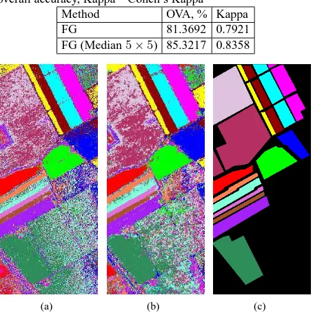
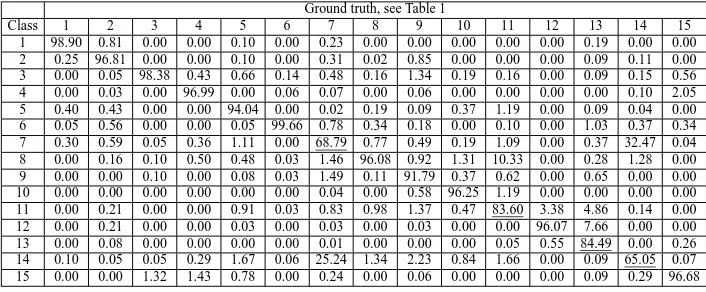
Table 2 presents the overall accuracy and Kappa coefficient for the classification. The additional experiment with feature median filtering allowed to obtain a better classification accuracy results (overall accuracy=85.3217 and Kappa=0.8358 versus 81.3692 and 0.7921, respectively; compare confusion Tables 3 and 4). Most of the classes were labeled with an accuracy more than 90%,
International Archives of the Photogrammetry, Remote Sensing and Spatial Information Sciences, Volume XXXIX-B7, 2012 XXII ISPRS Congress, 25 August – 01 September 2012, Melbourne, Australia
except several most difficult classes (these classes are usually hard to label and are mainly confused, see Tables 3 and 4). The classes 7 (Grapes untrained) and 14 (Vinyard untrained) illus-trate the highest confusion with classification accuracies equal to 68.79% and 65.05% (Table 4), respectively. Classes 11 (Let-tuce romaine 5wk) and 8 (Soil vinyard develop), also class 13 (Lettuce romaine 7wk) and 12 (Lettuce romaine 6wk) and 11 (Let-tuce romaine 5wk) are less confused.
Median filtering reduced the influence of the outlier samples in the input data for classification. Confusion among classes was re-duced and a better labeling was reached. MNF data preprocessing allows to reduce the time of calculation with a competitive clas-sification accuracy. On full bands set data a better clasclas-sification accuracy is expected to be obtained.
Approximate inference methods should be employed for the like-lihood probability computation. Approximate inference allows to calculate decisions with the accuracy comparable to the results of full propagation methods but with a high reduction of run time. In this work Mean Field approximate inference method was em-ployed. Factor graph allows to perform an inference for one class (to produce a probability map) leading to an application of mate-rial detection in hyperspectral data.
Among disadvantages we can note that probabilistic models re-quire computational time higher than many classification meth-ods, since inference in each point of input data is performed. Also maximum principle on the likelihood probability maps (per-formed to obtain class label map) can be a source of misclassifi-cation.
Table 2: The accuracy of salinas benchmark classification using the FG (MNF 20 features, alphabet size: 100). Additional ex-periment with feature median filtering is also presented. OVA – overall accuracy, Kappa – Cohen’s Kappa
Method OVA, % Kappa
FG 81.3692 0.7921
FG (Median5×5) 85.3217 0.8358
(a) (b) (c)
Figure 3: Classification maps for Salinas benchmark using factor graphs: (a) MNF, 20 features, alphabet size: 100, (b) MNF, 20 features, median filtering5×5, alphabet size: 100, (c) ground truth label map
4 CONCLUSIONS
The paper presents another successful area of factor graphs ap-plication: multispectral data classification. A relatively simple
structure of the FG allows to reach a competitive accuracy of classification even on data with decreased radiometric range (rep-resented on the alphabet). An important property of factor graph classification is that the method requires a relatively low number of training samples (only 20 points for a class). Separate process-ing of input features (spectral bands) and employment of the pre-sented data fusion and classification model is not influenced by the limitations of data dimensionality (i.e. there is no the curse of dimensionality). Classification on full data (all spectral bands) is possible to run (comparing to MNF features) and will take more computational time.
REFERENCES
Bishop, C., 2006. Pattern recognition and machine learning. In-formation Science and Statistics. Springer, New York.
Boardman, J. and Kruse, F., 194. Automated spectral analysis: a geological example using aviris data, north grapevine mountains, nevada. In: Proceedings of the Tenth Thematic Conference on Geological Remote Sensing, San Antonio, TX, USA, pp. 407– 418.
Bratasanu, D., Nedelcu, I. and Datcu, M., 2011. Bridging the se-mantic gap for satellite image annotation and automatic mapping applications. IEEE Journal of Selected Topics in Applied Earth Observations and Remote Sensing 4(1), pp. 193–204.
Frey, B. and Jojic, N., 2005. A comparison of algorithms for inference and learning in probabilistic graphical models. IEEE Transactions on Pattern Analysis and Machine Intelligence 27(9), pp. 1392–1416.
Green, A., Berman, M., Switzer, P. and Craig, M., 1988. A trans-formation for ordering multispectral data in terms of image qual-ity with implications for noise removal. IEEE Transactions on Geoscience and Remote Sensing 26(1), pp. 65–74.
Kschischang, F., Frey, B. and Loeliger, H.-A., 2001. Factor graphs and the sum-product algorithm. IEEE Transactions on Information Theory 47(2), pp. 498–519.
Lienou, M., Maitre, H. and Datcu, M., 2010. Semantic annota-tion of satellite images using latent Dirichlet allocaannota-tion. IEEE Geoscience and Remote Sensing Letters 7(1), pp. 28–32.
Wang, C., Blei, D. and Fei-Fei, L., 2009. Simultaneous image classification and annotation. In: IEEE Conference on Computer Vision and Pattern Recognition, pp. 1903–1910.
International Archives of the Photogrammetry, Remote Sensing and Spatial Information Sciences, Volume XXXIX-B7, 2012 XXII ISPRS Congress, 25 August – 01 September 2012, Melbourne, Australia
Table 3: Confusion matrix of the FG classification on Salinas benchmark (MNF 20 features, alphabet size: 100). Overall accu-racy=81.3692, Kappa=0.7921 Percentages are given for an easier interpretation.
Ground truth, see Table 1
Class 1 2 3 4 5 6 7 8 9 10 11 12 13 14 15 1 98.36 0.48 0.00 0.00 0.03 0.06 0.13 0.00 0.03 0.00 0.00 0.00 0.00 0.00 0.00 2 1.14 96.54 0.00 0.00 0.00 0.00 0.15 0.00 0.34 0.00 0.00 0.00 0.00 0.01 0.00 3 0.00 0.05 87.96 1.51 0.38 0.11 0.90 0.56 1.07 0.28 1.19 0.00 0.00 0.34 0.78 4 0.00 0.00 0.35 94.62 0.03 0.00 0.20 0.02 0.12 0.19 0.42 0.00 0.00 0.07 2.43 5 0.20 0.03 0.00 0.00 96.36 0.00 0.09 0.02 0.15 0.09 0.47 0.00 0.00 0.01 0.15 6 0.05 1.58 0.00 0.14 0.08 99.58 0.52 0.10 0.12 0.28 0.05 0.00 0.47 0.26 0.11 7 0.15 0.03 0.30 0.00 0.20 0.03 58.73 0.32 0.24 0.28 0.99 0.00 0.09 35.84 0.00 8 0.05 0.05 0.46 0.22 0.33 0.06 1.61 95.70 2.10 3.56 14.58 0.33 0.09 1.33 0.07 9 0.00 0.03 0.15 0.22 0.20 0.03 2.32 0.55 91.00 2.06 3.94 0.00 1.31 1.31 0.11 10 0.00 0.21 0.10 0.00 0.00 0.03 0.02 0.05 1.80 91.29 3.79 0.00 0.37 0.01 0.04 11 0.05 0.05 0.05 0.00 0.51 0.00 1.54 1.79 0.98 1.31 70.37 3.93 2.06 0.39 0.00 12 0.00 0.21 0.00 0.00 0.03 0.00 0.31 0.03 0.18 0.28 1.76 93.45 7.57 0.03 0.00 13 0.00 0.30 0.00 0.00 0.08 0.00 0.03 0.00 0.46 0.00 0.05 1.97 86.54 0.00 0.22 14 0.00 0.38 0.71 0.07 0.91 0.11 32.80 0.77 1.19 0.37 2.18 0.33 1.31 59.87 0.37 15 0.00 0.05 9.92 3.23 0.88 0.00 0.64 0.10 0.21 0.00 0.21 0.00 0.19 0.52 95.71
Table 4: Confusion matrix of the FG classification on Salinas benchmark (MNF 20 features, alphabet size: 100, feature median5×5 filtering). Overall accuracy=85.3217, Kappa=0.8358 Percentages are given for an easier interpretation.
Ground truth, see Table 1
Class 1 2 3 4 5 6 7 8 9 10 11 12 13 14 15 1 98.90 0.81 0.00 0.00 0.10 0.00 0.23 0.00 0.00 0.00 0.00 0.00 0.19 0.00 0.00 2 0.25 96.81 0.00 0.00 0.10 0.00 0.31 0.02 0.85 0.00 0.00 0.00 0.09 0.11 0.00 3 0.00 0.05 98.38 0.43 0.66 0.14 0.48 0.16 1.34 0.19 0.16 0.00 0.09 0.15 0.56 4 0.00 0.03 0.00 96.99 0.00 0.06 0.07 0.00 0.06 0.00 0.00 0.00 0.00 0.10 2.05 5 0.40 0.43 0.00 0.00 94.04 0.00 0.02 0.19 0.09 0.37 1.19 0.00 0.09 0.04 0.00 6 0.05 0.56 0.00 0.00 0.05 99.66 0.78 0.34 0.18 0.00 0.10 0.00 1.03 0.37 0.34 7 0.30 0.59 0.05 0.36 1.11 0.00 68.79 0.77 0.49 0.19 1.09 0.00 0.37 32.47 0.04 8 0.00 0.16 0.10 0.50 0.48 0.03 1.46 96.08 0.92 1.31 10.33 0.00 0.28 1.28 0.00 9 0.00 0.00 0.10 0.00 0.08 0.03 1.49 0.11 91.79 0.37 0.62 0.00 0.65 0.00 0.00 10 0.00 0.00 0.00 0.00 0.00 0.00 0.04 0.00 0.58 96.25 1.19 0.00 0.00 0.00 0.00 11 0.00 0.21 0.00 0.00 0.91 0.03 0.83 0.98 1.37 0.47 83.60 3.38 4.86 0.14 0.00 12 0.00 0.21 0.00 0.00 0.03 0.00 0.03 0.00 0.03 0.00 0.00 96.07 7.66 0.00 0.00 13 0.00 0.08 0.00 0.00 0.00 0.00 0.01 0.00 0.00 0.00 0.05 0.55 84.49 0.00 0.26 14 0.10 0.05 0.05 0.29 1.67 0.06 25.24 1.34 2.23 0.84 1.66 0.00 0.09 65.05 0.07 15 0.00 0.00 1.32 1.43 0.78 0.00 0.24 0.00 0.06 0.00 0.00 0.00 0.09 0.29 96.68
International Archives of the Photogrammetry, Remote Sensing and Spatial Information Sciences, Volume XXXIX-B7, 2012 XXII ISPRS Congress, 25 August – 01 September 2012, Melbourne, Australia