isprsarchives XXXIX B4 103 2012

VECTORIZATION OF LINEAR FEATURES IN SCANNED TOPOGRAPHIC MAPS

USING ADAPTIVE IMAGE SEGMENTATION AND SEQUENTIAL LINE TRACKING

Yun Yang a, *, Xiaoya An a, Limin Huang a

a

State Key Laboratory of Geoinformatic Engineering, Xi’an Research Institute of Surveying and Mapping, Xi’an,

710054, China - yytoall@126.com

KEY WORDS: Colour map, Vectorization, Sliding window, Image segmentation, Line tracking

ABSTRACT:

Vectorization of cartographic features is a difficult task in geographic information acquisition from topographic maps. This paper presents a semi-automatic approach to linear feature vectorization directly in original scanned colour topographic maps without layer separation. In the approach, a sliding window is added on a user-given linear feature, and the current line in the window is segmented adaptively by using colour space conversion, k-means clustering and directional region growing. A thinning operation is then performed in the window and the line is tracked from the centre to the edge. By moving the window continuously along the line, vectorization is carried out by iterative operations of image segmentation, thinning and line tracking. Experimental results show that linear features in colour topographic maps can be vectorized rapidly and accurately, especially in those maps with forest tints and relief shadings.

* Corresponding author.

1. INTRODUCTION

Map digitization is one of the most important means of geographic data acquisition for Geographic Information System (GIS) applications. In the past decades, map digitization has undergone the stage of manual tracking on digitizing tablets and the stage of heads-up screen digitizing. Currently, human-machine interactive digitization based on image processing and pattern recognition techniques has been more and more used.

Many commercial systems such as VPStudio, RxAutoImage, R2V and MapGIS are available for map digitization. Topographic maps are vectorized from raster images into vector data by raster-to-vector conversion. For black-and-white line drawings with high quality, automatic vectorization can be implemented by using line tracking method. However, for colour topographic maps, where cartographic features with different colours overlap and intersect one another, automatic vectorization is still a challenging task.

The existing techniques of colour map vectorization can be grouped into two main categories: colour segmentation based and original map based. The colour segmentation based method first split the colour map image into several layers with predefined map colours, and then vectorize cartographic features in the separated binary layers interactively or automatically. This kind of method can significantly reduce the complexity of cartographic features, and therefore make map vectorization relatively easy. Here, colour segmentation is a fundamental step. The precision and speed of map vectorization rely on the quality of segmented images. Many algorithms for colour segmentation including statistic pattern classification (Feng et al., 1996; Su et al., 1999), neural network (Lin et al., 1994; Guo et al., 1998), fuzzy clustering (Zheng et al., 2003), and others have been developed. Nevertheless, these algorithms are far from being satisfactory. Due to the influence of original paper map’s quality and the scanner’s performance, colours in a scanned map image are not the same as that in the original map. Large numbers of scattered colours and noises exist in the

image, especially for the map with forest tints and relief shadings. So it is difficult to segment the colour map image into perfect colour layers with high qualities. Noises, gaps and adhesions appear everywhere in the separated layers, particularly in the contour line layer. Although some algorithms for removing noises and connecting broken lines have been developed (Cheng et al., 2003; Zeng et al., 2004), a great deal of human editing is still inevitable to acquire high quality image for automatic vectorization.

Another way to vectorize linear features is based on original scanned colour maps. In this method, a linear feature is tracked starting from a user-specified point, and some kinds of flexible user interventions are allowed in case where automatic tracking fails. This approach utilizes the strategy of human-machine cooperation, makes the line tracking process under human control, and provides the ability to correct data immediately if required. Therefore, it is more practical for colour map vectorization, and can be used as a complimentary of the former method. It should be a preferred one for the map image with poor quality. Unfortunately, to the best of our knowledge, very few research works have been done on such vectorization method (Wu et al., 1998; Huang et al., 2005).

MapGIS is one of the most powerful GIS software systems produced by Zondy Cyber Group Co., LTD, which provides the way of interactive line tracking in original colour map images. In the process of line tracking, the minimum colour distance rule is adopted to determine the next tracking point. From the point of view of applications, this method has two main disadvantages in performance:

(1) The line tracking process depends greatly on the user-specified starting point. The user needs to magnify the image and select the midpoint of a line exactly as the starting point. If the selected point has a little deviation, the following line tracking cannot be ensured to be along the centreline.

(2) Automatic line tracking often fails when meeting other cartographic features with similar colour. Linear features can hardly be tracked in those maps with forest tints and relief shadings.

In order to overcome the above shortcomings, this paper presents a new technique for linear feature vectorization directly in colour map images. It is accomplished by using adaptive image segmentation and sequential line tracking based on sliding window.

2. THE ANALYSIS OF COLOR TOPOGRAPHIC MAP IMAGES

Topographic maps typically use only a few distinct colours to represent different cartographic feature layers, for example, black cultural features, brown geomorphologic features, blue water areas, green vegetation, and so on. Influenced by the RGB misalignment in the scanning process and the quality of the original map, large numbers of scattered colours and noises are generated in a scanned colour map. For instance, when a brown colour patch is scanned into a computer, many scattered colour pixels such as light brown, yellowish brown, dark brown are generated, which do not exist in the original map. In addition, cartographic features in different colours are more likely to overlap and intersect one another. These factors cause the phenomenon that features in the same layer do not have the same colour and similar colours do not represent the same feature layer, and therefore introduce great difficulty for colour segmentation based on colour information. Figure 1 shows a part of a colour topographic map with relief shadings and the result of segmented contour line layer. It shows that shading areas adhere together and a large number of broken lines occur in colour segmented layer. Therefore, automatic vectorization can not be performed at all in such low quality image.

(a) (b)

Figure 1. A part of a colour topographic map with relief shadings. a Original image. b The colour segmentation result of

contour line layer

3. THE PROPOSED APPROACH

The objective of our work is to find a way of vectorizing linear features directly in original colour map images without colour segmentation. How to distinguish linear features adaptively from the complicated background and how to track linear features rapidly are the key problems to be solved. In a colour topographic map image, different regions usually show marked differences in colour, brightness and contrast, especially those regions with forest tints and relief shadings. So it is difficult to distinguish linear features from the background using a global

method. Considering this, we propose a local adaptive segmentation method based on sliding window to separate linear features from background, followed by a sequential line tracking to vectorize linear features.

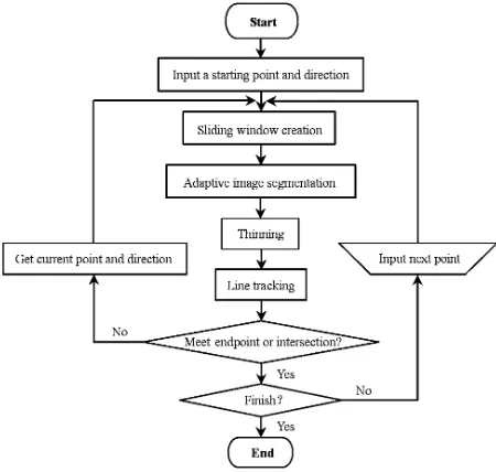
Figure 2 shows the procedure of linear feature vectorization. For a specified linear feature, a starting point and initial direction are first input by the operator, and a predefined rectangle window (which is called sliding window) is added on the line. Then, adaptive image segmentation, thinning, and line tracking are performed in the window. By moving the window continuously along the line and doing the above operations iteratively, the line is tracked sequentially until an endpoint or an intersection is met. If the tracking is broken or a tracking error occurs before arriving at the end of the line, manual operation is necessary to cross the intersection or move back to the correct position. After that, the sequential line tracking continues until the whole line has been vectorized.

Figure 2. The procedure of linear feature vectorization

3.1 Adaptive image segmentation based on sliding window

In this study, image segmentation aims at separating a specified linear feature from colour map image. The proposed approach is applied to the aforementioned sliding window, and is performed by using colour space conversion, k-means clustering and directional region growing.

3.1.1 Colour space conversion: Since there are numerous colours in a scanned colour map image, we first convert the colour image in the sliding window into a 256 grey-scale image so as to reduce the complexity of the problem. This is due to the following considerations: Firstly, colour confusion can be improved in the image with limited grey-scale. Secondly, it is relatively easy to separate objects from the grey-scale image because there is a marked contrast between foreground and background.

YIQ colour space is adopted here on account of its advantage of separating grey-scale information from colour data. In the YIQ colour space, image data consists of three components: luminance (Y), hue (I), and saturation (Q). The first component represents grey-scale information, while the last two components represent colour information. By converting an International Archives of the Photogrammetry, Remote Sensing and Spatial Information Sciences, Volume XXXIX-B4, 2012

RGB image into YIQ format, the grey-scale information can be extracted without loss(Chen et al., 2000).

The conversion from RGB to YIQ (Ford et al., 1998) can be expressed as

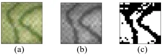
where Y component is the grey-scale value converted from RGB value. Figure 3a and 3b shows the colour image and the converted grey-scale image in a 25

×

25 sliding window of Figure 1a.

(a) (b) (c)

Figure 3. The image in a 25

×

25 sliding window. a Colour image. b Gray-scale image. c Segmentation by thresholding

3.1.2 Adaptive image segmentation: The commonly used segmentation approaches to grey-scale images include thresholding, feature space clustering, region growing, etc. Segmentation by thresholding is particularly useful for images containing objects resting upon contrasting background. But for a colour map image with many colour confusions, the converted grey-scale image may not have obvious valley in the histogram. So it is difficult to separate objects from background by using the theoretical optimal threshold, especially for the image with low contrast and low Signal-to-Noise Ratio (SNR). Figure 3c is the experimental result using Otsu thresholding method (Fu, 2001) for image segmentation. It can be seen that the lines in the window are bordered with noises and adhesions.

In order to achieve satisfying segmentation effect, this paper presents an adaptive image segmentation algorithm. The algorithm combines k-means clustering with directional region growing to segment the specified linear feature in the sliding window. First, k-means clustering is applied to a small neighbourhood (5

×

5) in the centre of the sliding window, and the pixels within the neighbourhood are divided into two regions of object and background. Then, the object region is expanded to the whole window by using directional region growing.. The reason why 5

×

5 neighbourhood is selected is that there are just only a single line in that small region, considering the line width and the distance between two lines in a topographic map image with a resolution of 300dpi. The neighbourhood should be correspondingly adjusted with the variation of linear feature width and the resolution of map image. K-means clustering is applied here because it is one of the simplest unsupervised learning algorithms for solving clustering problem (Wagstaff et al., 2001). K-means clustering and directional region growing are performed automatically in the sliding window no matter how the brightness changes, therefore it is an adaptive segmentation algorithm.

K-means clustering

The process of k-means clustering is as follows.

Step 1: Choose the pixel with minimum grey-scale as a seed within a 5

×

5 neighbourhood in the centre of the sliding window.

Step 2: Find the maximum and minimum grey-scale values in the 5

×

5 neighbourhood of the seed pixel, and let them be the initial clustering centre

c

₁ and

c

₂ of the object and background region respectively.

Step 3: For each pixel with grey-scale

g

_ij in the neighbourhood,

calculate

1

1 g c

d = ij − and d2 = gij −c2 . If

d

1

<

d

2, then

the pixel belongs to the object region, otherwise the background region.

Step 4: Calculate the average grey-scales m₁ and m₂ of the object and background region respectively. If they converge to

1

c

and

c

₂, the clustering ends; otherwise, let m₁ and

m

₂ be

the new clustering centre

c

₁ and

c

₂, go to Step 3.

Step 5: Set all the grey-scale values of the pixels belonging to the target region within the 5

×

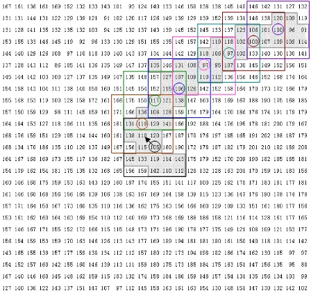
5 neighbourhood to be 1.

For the grey-scale matrix of Figure 3b, k-means clustering is performed in the 5

×

5 neighbourhood of the seed pixel (Its grey-scale value is 105). Figure 4 shows the object and background region after k-means clustering.

Figure 4. K-means clustering within a 5

×

5 neighbourhood

Directional region growing

Based on the k-means clustering result, directional region growing is performed in the whole sliding window. Before presenting the algorithm, the initial direction given by the operator is transformed into eight discrete directions d1, d2, …, d8 (as shown in Figure 5a), and the four sides of a 5×5

The directional region growing is described as follows.

Step 1: Initialization. International Archives of the Photogrammetry, Remote Sensing and Spatial Information Sciences, Volume XXXIX-B4, 2012

Find the pixel with minimum original grey-scale value along Li (i=1,3,5,7) within the target region as a new seed if the initial direction is di (i=1,3,5,7).

Find the pixel with minimum original grey-scale value along Li-1 and Li+1 (i=2,4,6,8; L8+1=L1 ) within the target region as a new seed if the initial direction is di (i=2,4,6,8).

Step 2: Perform k-means clustering within the 5 ×5 neighbourhood of the seed, obtaining new clustering centre

c

₁

and

c

₂.

Step 3: Find the pixels in the 5×5 neighbourhood meeting the following two rules, add them into the object region, and set their grey-scale values to be 1.

Rule 1. The grey-scale difference between the pixel and the object clustering centre is smaller than that between the pixel and background clustering centre, i.e.,

2

1

g

c

c

g

ij

−

<

ij

−

.

Rule 2. There is at least one pixel with binary value 1 in the 8-neighborhood.

Step 4: Find the pixel with minimum original grey-scale value in those pixels belonging to the newly grown target region at the four sides of the 5×5 neighbourhood as a new seed.

Step 5: Repeat Step2-Step4 until the edge of the sliding window is reached.

Step 6: Set the grey-scale values of pixels belonging to the background region to be 0.

After the above steps, the segmentation result in the sliding window is obtained (see Figure 6).

Figure 6. K-means clustering and directional region growing in the sliding window

3.2 Sequential line tracking

After image segmentation, a thinning operation is performed, followed by a line tracking process in the sliding window. By moving the window continuously along the line and doing the

above operations iteratively, the line is tracked sequentially until an endpoint or an intersection is met.

Before giving the algorithm, we first introduce several terms in binary thinned images (see Figure 7).

Endpoint：The point with one black pixel in the 3

×

3 neighbourhood.

Connecting point：The point with two black pixels in the 3

×

3 neighbourhood.

Crossing point：The point with more than three black pixels in the 3

×

3 neighbourhood.

(a) (b) (c)

Figure 7. a Endpoint. b Connecting point. c Crossing point

The sequential line tracking algorithm is described as follows.

Step 1: Find a connecting point P0 as the starting point in a

3

×

3 neighbourhood in the centre area of the sliding window.

Step 2: Select a point from the two black pixels in the 3

×

3 neighbourhood of P0 with a close direction d to the current

direction (The initial direction is input by a human operator).

Step 3: Make the current point invisible (set it to be white), and track to the next point Pi in direction d i is counted from 1 .

Step 4: Distinguish Pi in 3

×

3 neighbourhood. There are three

cases as follows.

If Pi is a connecting point, there remains only one black

pixel in its 3

×

3 neighbourhood but the invisible point, use its direction as tracking direction d, go to Step 3.

If Pi is a crossing point, judge that it is a true or pseudo

crossing point (more is said about this in the following). If it is true, stop tracking; otherwise, judge the forward direction d, go to Step 3.

If Pi is an endpoint or a side point of the sliding window, go

to Step 5.

Step 5: Count the number of the tracking points. If it is less than 3, stop tracking; otherwise, move the centre of the sliding window to the current point, and restart Step 1.

In the above process, crossing points may be encountered due to intersections between different linear features, or due to noise. The former is called true crossing point while the latter is called pseudo crossing point. When a true crossing point is met, automatic line tracking stops for a moment, and the next point is input manually. After that, the line tracking continues as before. When a pseudo crossing point is met, an automatic judgment of forward direction is needed to across the pseudo crossing point.

To handle the pseudo crossing point, a concentration degree

∑

fijis defined, which means the total number of black pixels

within a limited region. Suppose that S is the point in the un-thinned binary image corresponding to the crossing point P. If the concentration degree around S is larger than a preset value, then P is treated as a true crossing point. Otherwise it is a pseudo one. For topographic maps with resolution of 300 dpi, International Archives of the Photogrammetry, Remote Sensing and Spatial Information Sciences, Volume XXXIX-B4, 2012

the concentration degree can be set as 20 within a 5

×

5 region. When meeting a pseudo crossing point, a trial-tracking is done to determine the next tracking direction. As shown in Figure 8, there are two forward directions d1 and d2 at the pseudo crossing point P. First, three connecting pixels along d1 and d2 are tracked respectively, and each of their corresponding grey-scale values in the grey-grey-scale image are recorded. Then, the average grey-scale values are calculated for d1 and d2, respectively. If the former is smaller, d1 is determined as the next tracking direction, else d2.

Figure 8. Determination of the forward direction at a pseudo crossing point

Figure 9 illustrates the continuous sliding window and sequential line tracking from the starting point with an initial direction pointed by the arrow. Figure 10 shows the results of image segmentation, thinning and line tracking in window 1-6 in Figure 9a. The grey line marked in each window draws a tracking path. By connecting all the grey lines in order, the tracking result is obtained (see Figure 9b).

(a) (b)

Figure 9. Sequential line tracking. a Continuous sliding window. b The result of line tracking

(a)

(b)

(c)

Figure 10. a Images in window 1-6 in Figure 9a. b Corresponding segmentation results of current linear feature. c Corresponding results of thinning and line tracking

4. EXPERIMENTS AND ANALYSIS

Experiments have been conducted to test our proposed method. Figure 11a is a part of a topographic map with relief shadings. The size of the image is 300

×

300 pixels, the resolution is 300 dpi, and the sliding window is 25

×

25 pixels. For each contour line, once a starting point and direction are input by a human operator, it can be tracked automatically. In the case that an intersection or a gap is met, automatic tracking stops, and a new point in the front is input manually. After that, the line tracking continues. If the gap is wider, a few points should be collected manually to get over it, and then automatic tracking resumes. Figure 11b is the vectorization result of contour lines. Figure 12a is a part of another topographic map with forest tints. The image size, the scanning resolution, and the window size remain unchanged. Figure 12b is the vectorization result of contour lines. The average time of vectorizing contour lines in Figure 11 and Figure 12 are 200 seconds and 160 seconds respectively on a 3 GHz Pentium (R) 4 computer. Most of the time was taken by manual input of starting points and some interventions during the tracking process, while the time required by automatic tracking is negligible.

(a) (b)

Figure 11. A part of a scanned colour topographic map with relief shadings. a Original image. b Vectorization result of

contour lines

(a) (b)

Figure 12. A part of another topographic map with forest tints. a Colour scanned image. b Vectorization result of contour lines

A mass of other maps including colour, grey and black-and-white maps have been vectorized, and satisfactory results have been achieved. The experiments shows that the proposed method is of great practical value in vectorizing linear features directly in original topographic map images especially those colour maps with forest tints and relief shadings.

Furthermore, a comparison with commercial software MapGIS has been made. For scanned colour maps with clear contrast International Archives of the Photogrammetry, Remote Sensing and Spatial Information Sciences, Volume XXXIX-B4, 2012

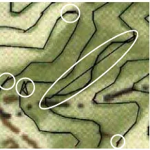
between topographic features and background, it took nearly the same time to vectorize linear features by using our method and MapGIS. But for map images with low contrast and low SNR, our method is obviously efficient. It took about 9 minutes to vectorize counter lines in Figure 11 by using MapGIS, apparently slower than our method. Tracking errors (as shown in the white circle marked areas in Figure 13) often occur in the process of vectorization, and more human interventions are needed to handle these problems.

Figure 13. Vectorization result of Figure 11 by MAPGIS ( locally enlarged

From the experiments, the proposed method demonstrates the following advantages:

(1) Most of the work of line tracking can be finished automatically while human operators only need to give the starting point and the directional point. Some kinds of manual interventions are allowed in case automatic tracking fails, which makes line tracking under human control, and provides the ability to correct data immediately if required.

(2) Linear features can be tracked accurately along the centerline after image segmentation and thinning. This can avoid deviation from the centerline using only colour distance to determine the tracking point.

(3) The sliding window is updated continuously and the segmentation result in each window depends on the grey-level distribution and spatial relationship of pixels in current window. This makes line tracking adapt to colour variations in light and shade areas.

5. CONCLUSION

This paper presents a method for linear feature vectorization directly in scanned colour maps. It has been proved to be valid and practical, especially for those maps with forest tints and relief shadings. The process of sliding window creation, adaptive image segmentation, thinning and sequential tracking can be used as general steps for colour map vectorization. Future improvement mainly focuses on automatic tracking across the intersections of different linear features so as to reduce human intervention and improve the speed of vectorization.

References

Cheng Qimin, Yang Chongjun, Shao Zhenfeng, 2003. Automatic Color Separation and Processing of Scanned Color Contour Maps. Journal of Geomatics, 28(5), pp. 4-6 (in Chinese)

Chen Zeyu, Qi Feihu, Chen Gang, 2000. Human Face Detection Using Color Information. Journal of Shanghai Jiaotong University, 34(6), pp. 793-795 (in Chinese)

Feng Yucai, Song Enmin, 1996. An Algorithm to gather colors from image of color maps. Journal of Software, 7(8), pp. 466-470 (in Chinese)

Ford A, Roberts A, 1998. “Colour Space Conversions”. http://www.poynton.com/PDFs/coloureq.pdf (16 April. 2012)

Fu Zhongliang, 2001. The Threshold Selection Method Based on the Measure of Difference between Images. Journal of Computer Research and Development, 38(5), pp. 563-567 (in Chinese)

Guo Zihua, Zhuang Zhenquan, 1998. Map Vectorization Algorithm Based on Gas. Journal of China University of Science and Technology, 28(4), pp. 476-481 (in Chinese)

Huang Zhili, Fan Yangyu, Hao Chongyang, 2005. Interactive Vectorization for Chromatic Scan Map. Computer Application, 25(3), pp. 577-579 (in Chinese)

Lin Hua, Wang Zhengguang, 1994. The Application of the ART Network in the Color Classification of Maps. Journal of Xidian University, 21(4), pp. 419-425 (in Chinese)

Su Haihua, Wang Ruibin, Zhuang Zhenquan, 1999. A Colour Segmentation Algorithm Applied in Maps with Its Implementation. Journal of Computer-aided Design &Computer Graphics, 11(5), pp. 395-398 (in Chinese)

Wagstaff K, Cardie C, Rogers S, et al, 2001. Constrained K-means Clustering with Background Knowledge. In: Proceedings of the Eighteenth International Conference on Machine Learning, Massachusetts, USA, pp. 577-584

Wu Xincai, Wang Xiaorui, 1998. The Method of Interactive Vectorization Based on Color Map. Mini-Micro Systems, 19(5), pp. 36-39 (in Chinese)

Zeng Yingsheng, Feng Jinguang, He Hangen, 2004. A Categorizing Algorithm in the Recognition of Contour Line. Computer Engineering and Application, 40(3), pp. 56-57+62 (in Chinese)

Zheng Huali, Zhou Xianzhong,Wang Jianyu, 2003. Research and Implementation of Automatic Color Segmentation Algorithm for Scanned Color Maps. Journal of Computer-aided Design &Computer Graphics, 15(1), pp. 29-33 (in Chinese)

Acknowledgements

The authors would like to thank Zondy Cyber Group Co., LTD for providing MAPGIS K9 to do the experiments.