*Corresponding author. Tel.: 31-13-4662028; fax: 31-13-4663280. E-mail address:[email protected] (A. van Soest).
Journal of Econometrics 101 (2001) 71}107
An analysis of housing expenditure using
semiparametric models and panel data
Erwin Charlier
!,"
, Bertrand Melenberg
!
, Arthur van Soest
!,
*
!Department of Econometrics, Tilburg University, P.O. Box 90153, 5000 LE, Tilburg, Netherlands"NIB Capital Asset Management, P.O. Box 8285 3503 RG, Utrecht, Netherlands Received 1 April 1997; received in revised form 1 March 2000; accepted 5 July 2000
Abstract
In this paper we model expenditure on housing for owners and renters by means of endogenous switching regression models for panel data. We explain the share of housing in total expenditure from a household speci"c e!ect, family characteristics, constant-quality prices, and total expenditure, where the latter is allowed to be endogenous. We consider both random and"xed e!ects panel data models. We compare estimates for the random e!ects model with estimates for the linear panel data model in which selection only enters through the "xed e!ects, and with estimates allowing for "xed e!ects and a more general type of selectivity. Di!erences appear to be substantial. The results imply that the random e!ects model as well as the linear panel data model are too restrictive. ( 2001 Elsevier Science S.A. All rights reserved.
JEL classixcation: C14; C33; R21
Keywords: Sample selection; Engel curves; Semiparametric models; Panel data
1. Introduction
In most industrialized countries housing is one of the main categories of household expenditure. Its understanding is, therefore, crucial for analyzing
household consumption. The decision how much to spend on housing is strongly related to the choice between renting and owning. The standard reference is Lee and Trost (1978), who explain annual family expenditure on housing taking the decision to own or to rent explicitly into account. They use cross-section data and apply a switching regression model with endogenous switching and normally distributed error terms, which is also referred to as Tobit V by Amemiya (1984). A recent application of this model is, for example, given by Megbolugbe and Cho (1996), who explain racial di!erences in housing demand of US families.
Several authors have focused on di!erent aspects of the demand for housing. Ioannides and Rosental (1994) analyze the choice between renting and owning in relation to consumption and investment demand for housing. Zorn (1993) models the fact that some households cannot obtain a mortgage due to mort-gage constraints, which results in a kinked budget set. Haurin (1991) also considers mortgage constraints, and analyzes how the intertemporal variation in income a!ects tenure choice. Ermisch et al. (1996) use cross-section data to analyze housing demand in Britain, using a switching regression model for recent movers vs. nonmovers. These authors focus on estimating price and income elasticities, and also compare their "ndings with earlier results for the US and the UK. They "nd income elasticities of around 0.5, which is rather low compared to the range of earlier estimates for the US (0.7}1.5) or the UK (0.5}1.1). The price elasticities they "nd are about
!0.4, which is again somewhat low compared to US "ndings (a range of
!0.8 through!0.5), but in line with earlier UK "ndings. They emphasize the sensitivity of their elasticity estimates for selectivity issues and the income measure.
In a series of studies, Axel BoKrsch-Supan and various coauthors analyze both cross-section and panel data models for housing choice in the US and Germany. See, for example, BoKrsch-Supan (1986, 1987), BoKrsch-Supan and Pitkin (1988), and BoKrsch-Supan and Pollakowski (1990). They focus on discrete choice models, using generalizations of the multinomial logit model. For example, BoKrsch-Supan and Pollakowski (1990) estimate a "xed e!ects multinomial logit model for the choice between four types of dwelling, distinguishing owner occupied vs. rental dwellings, and large vs. small dwellings.
In this paper we focus on housing expenditure and not on housing assets, housing equity or mortgage constraints. Thus, our dependent variable is con-tinuous instead of discrete, so that we cannot use BoKrsch-Supan's discrete choice type of panel data models. We will combine the model of Lee and Trost (1978), henceforth referred to as LT model, with the consumer demand literature on expenditure on goods. We extend the LT model in two ways. First, we use panel data, and can therefore allow for time constant unobserved household speci"c e!ects which can be correlated with the regressors. In other words, we will allow
for "xed e!ects, which would be impossible in the cross-section context. The usual cross-section model imposes independence between individual e!ects and regressors or instruments, which, in a panel data context, leads to the more restrictive random e!ects model. There are two types of "xed e!ects models that we consider: a linear model in which selectivity only enters through the "xed e!ects, and a model similar to that of Kyriazidou (1997), which incorporates more general selectivity e!ects than the linear model. We will compare results for these two"xed e!ects models with those of a random e!ects model.
Following the two-stage budgeting consumption literature (Blundell and Walker, 1986), we will explain housing expenditure from total expenditure rather than income. A second generalization compared to the LT model, is that we take account of potential endogeneity of total expenditure. We test for this and present estimates allowing for it. Our main focus is the sensitivity of housing expenditure for total expenditure and for prices. We construct and incorporate prices along the lines of BoKrsch-Supan (1987) and BoK rsch-Supan and Pollakowski (1990), exploiting price variation across time and across space.
Our main "ndings are that the random e!ects model, the model in which selectivity enters through the"xed e!ects only, and the model which assumes that total expenditure is exogenous, are all rejected against the more general
"xed e!ects model. Moreover, the models lead to di!erent conclusions about aggregate elasticities of housing expenditure with respect to total expenditure and prices.
The remainder of this paper is organized as follows. In Section 2 we de-scribe the data, drawn from the Dutch Socio Economic Panel, 1987}1989. In Section 3 we discuss various parametric and semiparametric panel data models and report our estimation and testing results using these models in order to explain housing. Section 4 concludes.
2. Data
We will use data from the waves 1987}1989 of the Dutch Socio-Economic Panel (SEP). Although this panel exists since 1984, information concerning housing is only present since 1986 and wealth data are available as of 1987. We will use a cleaned subsample for each year with information on family character-istics (including marital status, number of children living with the family, age of the head of household, education level and region of residence), and labor market characteristics (including hours of work, gross and net earnings). The labor market characteristics are used to construct household income which consists of labor earnings, other family income (mainly from letting rooms or child allowances), bene"ts and pensions. Personal income of children is
1Net wealth is constructed using checking accounts, savings and deposits accounts, saving certi"cates, certi"cates of deposits, bonds and mortgage bonds, shares, options and other securities, antiques, jewels, coins, etc., real estate other than one's own residence, one's own car, claims against private persons, other assets, life-insurance with saving elements, personal loan or revolving credit, hire-purchase and other loans.
2We also corrected for donations, bequests, and capital gains.
3Mortgage interest payments are tax deductible. See Appendix A for computation of the marginal tax rate.
4This refers to a direct tax on housing property and to extra income tax due to adding the imputed rental value of the house to household income.
excluded. Asset income and capital gains are also excluded, because this type of income is strongly related to the home ownership decision. Wealth data1are used to construct savings.2For issues on cleaning the savings data we refer to Camphuis (1993). Income and savings are used to construct total expenditure. Expenditure and income are reported inDutch guilders per month.
The budget share spent on housing is de"ned as the fraction of total expendi-ture spent on housing. Housing expendiexpendi-ture for renters is the amount of money spent on rent by the family (i.e., excluding gas/water/electricity/heating as well as rental subsidy). For owners expenditure on housing consists of the following components: net interest costs on the mortgage,3net rent paid if the land is not owned, taxes on owned housing,4costs of insuring the house, opportunity costs of housing equity, maintenance costs, and minus the increase of the value of the house. The latter three costs components are not observed in the data. The opportunity cost of the foregone interest on housing equity is set equal to 4% of the value of the house minus the mortgage value. Maintenance costs and the increase of the value of the house are set equal to 2% and 1% of the value of the house, respectively. In Appendix A, we shall investigate the sensitivity of the results with respect to these choices. It appears that most results are hardly a!ected.
Appendix A contains some further details on the construction of the sample and the variables of interest, and a comparison with macro-data on housing expenditure. Given this sample, we excluded households with item nonresponse on wealth or income, implying that total expenditure is missing, and we also excluded a few households with housing budget share larger than 0.6. For the 1987 wave this reduces the dataset from 3006 to 2273 observations. In addition to the data derived from the SEP, we also included constant-quality prices of owned and rented housing, constructed along the lines of BoKrsch-Supan (1987) and BoKrsch-Supan and Pollakowski (1990). These prices vary over time and space; Appendix A contains the details.
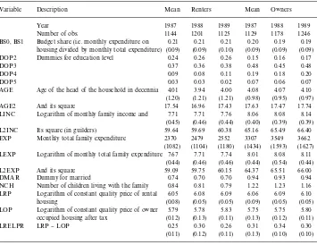
Variable de"nitions and summary statistics for the three resulting panel waves are presented in Table 1. The average budget share of housing is 0.21 for
Table 1
Overview of variables and summary statistics for 1987, 1988 and 1989 (standard deviations in parentheses)
Variable Description Mean Renters Mean Owners
Year 1987 1988 1989 1987 1988 1989 Number of obs. 1144 1201 1125 1129 1178 1246 BS0, BS1 Budget share (i.e. monthly expenditure on 0.21 0.21 0.21 0.20 0.19 0.19 housing divided by monthly total expenditure) (0.09) (0.09) (0.10) (0.09) (0.09) (0.09) DOP2 Dummies for education level 0.24 0.26 0.26 0.15 0.16 0.17
DOP3 0.37 0.36 0.38 0.48 0.45 0.48
DOP4 0.09 0.08 0.11 0.19 0.18 0.20
DOP5 0.03 0.03 0.02 0.07 0.06 0.07
AGE Age of the head of the household in decennia 4.01 3.94 4.00 4.08 4.07 4.10 (1.20) (1.21) (1.21) (0.98) (0.95) (0.97) AGE2 And its square 17.54 16.96 17.43 17.63 17.47 17.74 LINC Logarithm of monthly family income and 7.71 7.71 7.76 8.06 8.08 8.14 (0.45) (0.46) (0.44) (0.40) (0.39) (0.39) L2INC Its square (in guilders) 59.64 59.69 60.38 65.16 65.49 66.40 EXP Monthly total family expenditure 2370 2479 2552 3307 3549 3662 (1082) (1104) (1180) (1434) (1593) (1627) LEXP Logarithm of monthly total family expenditure 7.67 7.71 7.74 8.01 8.08 8.11
(0.44) (0.46) (0.46) (0.44) (0.54) (0.44) L2EXP And its square 59.09 59.75 60.15 64.37 65.51 66.00 DMAR Dummy for married 0.74 0.70 0.70 0.94 0.93 0.94 NCH Number of children living with the family 0.84 0.81 0.79 1.22 1.23 1.16 LRP Logarithm of constant quality price of rental 6.05 6.08 6.09 6.06 6.09 6.10 housing (0.08) (0.05) (0.05) (0.09) (0.05) (0.05) LOP Logarithm of constant quality price of owner 5.79 5.78 5.83 5.75 5.75 5.80
occupied housing after tax (0.12) (0.13) (0.11) (0.13) (0.12) (0.11) LRELPR LRP}LOP 0.25 0.30 0.26 0.31 0.34 0.30
(0.11) (0.12) (0.11) (0.13) (0.10) (0.10)
renters and about 0.20 for owners. For owners, this share decreased slightly over time.
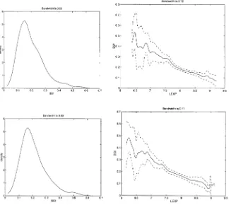
Figs. 1 and 2 describe the 1987 data in some more detail. In Fig. 1, non-parametric density estimates for the budget shares BS0 for renters and BS1 for owners are shown, as well as nonparametric regressions of these budget shares on log(total expenditure). Both budget share distributions are skewed to the right. The regression estimates suggest that the housing budget share is nonlin-ear in log(total expenditure), but can be approximated reasonably well by a quadratic function. This is similar to what Banks et al. (1994)"nd for many commodity groups.
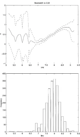
In Fig. 2, the result of a nonparametric regression of the probability of owning a house as a function of log(total income) is presented together with the frequency distribution of log(total income). Families with higher total income tend to have a higher probability of owning a house for the main part of the income range.
Fig. 1. Nonparametric density estimates for BS1 and BS0 and nonparametric regression estimates of the same variables on log total expenditure (LEXP), together with 95% uniform con"dence bands.
3. Models
The panel data models we consider allow for household speci"c e!ects which are either assumed to be independent of the explanatory variables (random e!ects), or allowed to be correlated with the explanatory variables ("xed e!ects). Starting point is the following system of equations:
d
it"1(n@xit#gi!uit*0), y
0it"b@0xit#a0i#e0it ifdit"0, y
1it"b@1xit#a1i#e1it ifdit"1.
Here the indicesiandtrefer to householdiin periodt(t"1,2,¹).ditis a sector
selection dummy variable, representing the tenure choice between owning and renting, which is 1 for owners and 0 for renters,x
Fig. 2. Nonparametric estimates of the probability of owning a house as a function of log household income (LINC), and distribution of LINC.
5The only exception we know of is given by Chen (1999). He relaxes the exclusion restriction and imposes an additional symmetry condition on the errors.
variables (log total expenditure and its square, prices, and taste shifters),y 0itand y
1itare the budget shares spent on housing for renters and owners, respectively. a
0i,a1i, and gi are unobserved household speci"c time-invariant e!ects, and e
0it,e1it, and uit are the error terms. b1,b0 and p are vectors of unknown
parameters. 1()) stands for the usual indicator function.
3.1. Random ewects
In a random e!ects model, wherea
0i,a1i,gi,e0it,e1it, and uit are normally
distributed and independent of x
it, we could apply the estimation procedure
proposed by Vella and Verbeek (1999). However, their estimation procedure relies on the normality assumptions. An alternative approach to estimate the slope parameters in the random e!ects panel data model is to consider each wave of data separately (i.e., three cross-sections). Considering a particular wave, we can drop thet-subscript, and include the random e!ects in the error terms which then becomev
i"(a0i#e0i,a1*#e1*,gi!ui); subsequently, we can use
existing estimation techniques for a cross-section endogenous switching regres-sion model. A semi-parametric cross-section model estimator gives consistent estimates for the slope parameters in the three equations (for each wave), without requiring normality of the errors.
Even if the error terms in a cross-section endogenous switching regression model are independent of the regressors, identi"cation of the parameters of this model, without further distributional assumptions, requires that at least one component of bothb1andb0are equal to zero (possibly the same), while the corresponding components ofn are not equal to zero. Such exclusion restric-tions are not required if normality of the errors is imposed, but are generally needed in a semi-parametric framework.5 Therefore, we will impose them throughout.
From an economic point of view, it is natural to exclude the price of rented housing from the housing demand equation for owners, and to exclude the price of owned housing from the demand equation for renters. Once the choice between renting and owning is made, the price of the alternative which is not chosen is no longer relevant. Another exclusion restriction we use is that the head of household's education level is not included in the budget share equa-tions. Education level may a!ect the family's information set and interest in
"nancial matters, and may, therefore, in#uence the family's portfolio choice, of which the choice between owning and renting is an important component. However, it is not clear why education should have a direct impact on housing
6See Blundell and Walker (1986), for example.
7Not all semiparametric estimators developed so far are also computationally convenient, in particular not those estimators which require optimization of a heavily nonlinear objective function with possibly many local optima.
consumption, given the ownership decision. Finally, we exclude the number of children from the share equations. Although there is no a priori reason for this, the number of children was always insigni"cant in the share equations at any conventional level.
As mentioned above, x
i will include the log of total expenditure and its
square, which might be endogenous. For example, according to the two-stage budgeting literature6a household"rst decides how much to spend in total in each period and, given this decision, it decides how much of this to spend on food, clothing, housing, etc. Thus, total expenditure per period is a decision variable and could be endogenous. In the model, where error terms arise due to future uncertainty only, total expenditure is exogenous to the share equations. However, introducing random preferences in a life-cycle consistent way will lead to a model in which the resulting error term is correlated with total expenditure so that total expenditure may be endogenous.
To the best of our knowledge, computationally convenient semi-parametric estimators of the model allowing for endogenous regressors in the binary choice selection equation are not available yet.7 Therefore, we shall assume that the log of total expenditure and its square are not present in the selec-tion equaselec-tion. Instead, this equaselec-tion includes the log of household income and its square, which can be seen as instruments for the total expenditure variables.
We decomposex
iintoxai, containing log total expenditure and its square,xbi,
containing log household income and its square, andx
di, containing prices and
taste shifters. Exclusion restrictions yieldx
cias a subvector ofxdi.xbiandxdiare
included in the selection equation, andx
ai and xci are included in the budget
share equations. The random e!ects assumption implies that the error terms
a0i#e
0i,a1i#e1i and gi!ui are assumed to be independent of (x@bi,x@di)@,
whereasx
a* is allowed to be endogenous.
A detailed analysis of various cross-section models is given in Charlier et al. (2000). Since in that paper, the normality assumption on (a
0i#e0i, a1i#e1*,
g
i!ui)@ is strongly rejected, we here only report the results based on the
approach of Newey (1988). This approach yields consistent estimators under weaker distributional assumptions than normality, and has the advantage of computational convenience. Newey's approach consists of two steps. The"rst step is to estimate the binary choice selection equation by maximum likelihood. In our search for a#exible enough speci"cation for this, we have experimented
8LM tests similar to those in Chesher and Irish (1987), reject normality in the extended probit model only for 1987. Homoskedasticity, however, is rejected for all waves, suggesting that the single index speci"cation might be inadequate, despite the seemingly high#exibility. Because Newey's estimator applies only to a single-index selection equation, alternative single-index semiparametric estimators are unlikely to perform much better.
with several single index generalizations of a probit model (see Appendix C), and found the following one-parameter extension:
PMd
i"1Dxbi,xdiN"U(n@bxbi#n@dxdi#q[n@bxbi#n@dxdi]2).
We also estimated the model with higher-order polynomials or rational functions of the single index, but these higher-order terms turned out to be in-signi"cant.
The second step is to estimate the budget share equations, taking account of selectivity bias and potential endogeneity of expenditure variables. Selection is accounted for by adding an extra regressor which can be seen as a correction term. This correction term is an unknown function of the indexn@bx
bi#n@dxdi.
The unknown function is replaced by a polynomial with coe$cients to be estimated, and the parameters nb and nd are replaced by their "rst round estimates. Newey shows that, for the case of exogenous regressors, OLS on the two subsamples with the terms of the polynomials added as additional re-gressors, leads to consistent estimates if the order of the polynomial tends to in"nity with the number of observations. He also derives the asymptotic covariance matrix of the estimator and a consistent estimate for it.
Potential endogeneity ofx
ai can be accounted for by using IV (withxci and
log family income and its square as instruments) instead of OLS in the second step. This is described extensively in Charlier et al. (2000). To make the current paper self-contained, we have included the details of this estimator and its implementation (choice of smoothing parameters, etc.) in Appendix C.
Results on the selection equation are presented in Table 2. In the left panel we present the ML estimates of the selection equation for each of the three waves separately. The estimate ofq, the coe$cient of (n@bx
bi#n@dxdi)2, is always
nega-tive, and signi"cant at the 5% level in the"rst and third wave. The results for the three waves are quite similar to each other. We "nd that the probability
PMd
i"1Dxbi,xdiNincreases with the indexn@bxbi#n@dxdiover the sample range.8
The income pattern is U-shaped, and the probability of ownership increases with income over most of the income range. The education e!ect is also positive, signi"cant, and much stronger than the income e!ect. The age pattern is inversely U-shaped with a maximum probability of ownership at about 45 years of age. Being married increases the probability of ownership; the number of children is insigni"cant. The regional dummies imply that ownership is higher in other regions than in the west of the country, where house prices are higher than elsewhere.
Table 2
Estimation results for the selection equation (standard errors in parentheses)!
Variable 1987, probit 1988, probit 1989, probit Pooled, probit 1987, logit Fixed e!ects logit
CONSTANT 33.506" (4.569) 9.669" (3.528) 15.552" (5.846) 12.897" (1.981) 54.583" (7.598) DOP2 0.170# (0.081) 0.071 (0.086) 0.274" (0.091) 0.166" (0.049) 0.288# (0.137) DOP3 0.480" (0.074) 0.361" (0.075) 0.548" (0.085) 0.460" (0.044) 0.802" (0.125) DOP4 0.566" (0.126) 0.527" (0.113) 0.616" (0.118) 0.580" (0.067) 0.952" (0.210) DOP5 0.483# (0.224) 0.280 (0.169) 0.594# (0.207) 0.478" (0.110) 0.835# (0.371)
AGE 1.185" (0.225) 1.443 (0.231) 1.456" (0.233) 1.358" (0.131) 2.024" (0.380) 16.875# (5.942)
AGE2 !0.126" (0.026) !0.160" (0.027) !0.160" (0.027) !0.149" (0.015) !0.217" (0.044) !2.091# (0.739)
LINC !10.591" (1.215) !4.515" (0.919) !6.017" (1.521) !5.282" (0.524) !17.304" (2.026) 6.590 (13.318)
L2INC 0.743" (0.080) 0.352" (0.061) 0.443" (0.099) 0.398" (0.035) 1.214" (0.134) !0.496 (0.838) DMAR 0.485" (0.090) 0.576" (0.099) 0.649" (0.095) 0.572" (0.054) 0.839" (0.156)
NCH 0.045 (0.034) 0.049 (0.031) 0.016 (0.033) 0.038# (0.018) 0.071 (0.056) !0.200 (0.497)
LRELPR 1.255" (0.296) 0.504 (0.282) 0.801# (0.306) 0.713" (0.162) 2.006" (0.496) 2.010 (2.604)
q !0.215" (0.021) !0.036 (0.061) !0.114# (0.049) !0.111" (0.027) !0.130" (0.014)
Dummy87 !2.682" (0.680)
Dummy88 !1.468" (0.459)
!Columns 2}6 are based on (pooled) cross-section data, column 7 is based on panel data and a model with"xed e!ects.
"Signi"cant at the 1% level.
#Signi"cant at the 5% level.
E.
Charlier
et
al.
/
Journal
of
Econometrics
101
(2001)
71
}
107
9The"nal column of Table 2 will be discussed in the next subsection.
10Results in Appendix B show that the results of the Newey (1988) estimates are not sensitive with respect to the de"nition of the expenditure measure for owners.
We have imposed that the coe$cients of the log prices for rented and owned housing add up to zero, implying that only the price ratio matters. The log of the price ratio of rental housing and owner occupied housing (LRELPR) has a positive e!ect, implying that a higher relative price of renting increases the probability of owning. This is in line with what one might expect.
For the sake of comparison we also included in Table 2 estimates based on pooled data for the three waves. We considered the cases without and with time dummies included. Since the time dummies turned out to be insigni"cant, we only report the estimation results without the time dummies. The estimates are always in the range of the estimates based on the three separate waves. Standard errors are generally lower than those for the three waves separately, and all pooled estimates are signi"cant at the 5% level. The conclusions do not change. In Table 2 we also make a comparison with a logit speci"cation instead of probit. We present the results for the 1987 wave. Taking into account the di!erences in normalization, the estimation results turn out to be quite similar.9
Results on the budget share equations are presented in Tables 3 and 4. Table 3 contains the results ignoring selection, while Table 4 presents the results taking selection into account. These tables also contain corresponding results for the
"xed e!ects models, to be discussed in the next subsection. The semiparametric estimates based upon Newey (1988) are presented in the upper panel of Table 4. We distinguish between the case in which LEXP and L2EXP are assumed to be exogenous, and the case where they are allowed to be endogenous.10 In both cases we calculated the series approximation of the correction term up to nine terms. Generally, for both owners and renters, the results did not change much after including seven terms in the series approximation.
The estimated standard errors, which take into account the"rst stage estima-tion error in the parameters of the selecestima-tion equaestima-tion, appear to di!er substan-tially from the standard OLS standard error estimates, but are similar to the Eicker-White standard errors. This indicates that the "rst stage errors hardly a!ect the standard errors of the second stage estimates, but that taking into account heteroskedasticity due to the selection correction term is crucial.
The results based on the pooled data are presented in Table 3 (no selection correction) and the bottom panel of Table 4 (with selection correction). When selectivity was taken into account we used seven terms in the series approxima-tion. We"nd that the standard errors increase substantially when endogeneity of LEXP and L2EXP is taken into account. Still, in the model which does not account for selectivity, all parameters remain signi"cant. Taking account of selectivity also leads to higher estimated standard errors. When both selectivity
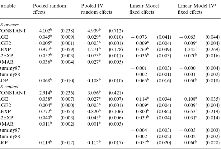
Table 3
Estimation results for the budget share equations without correction for selection (standard errors in parentheses)
Variable Pooled random e!ects
Pooled IV random e!ects
Linear Model "xed e!ects
Linear Model IV!
"xed e!ects BS owners
CONSTANT 4.102" (0.238) 4.939" (0.712)
AGE 0.045" (0.009) 0.029" (0.010) !0.073 (0.041) !0.063 (0.044) AGE2 !0.005" (0.001) !0.003" (0.001) 0.009" (0.004) 0.009# (0.004) LEXP !0.977" (0.059) !1.271" (0.178) !0.769" (0.049) !1.345" (0.269) L2EXP 0.052" (0.003) 0.073" (0.011) 0.036" (0.003) 0.070" (0.016) DMAR 0.036" (0.004) 0.027" (0.005)
Dummy87 !0.001 (0.003) !0.000 (0.004)
Dummy88 !0.002 (0.001) !0.001 (0.002)
LOP 0.068" (0.010) 0.108" (0.010) 0.065" (0.016) 0.050" (0.018) BS renters
CONSTANT 2.914" (0.236) 3.056" (0.421)
AGE 0.038" (0.007) 0.027" (0.007) 0.114" (0.034) 0.108" (0.035) AGE2 !0.004" (0.000) !0.003" (0.001) !0.009# (0.004) !0.009# (0.004) LEXP !0.772" (0.055) !0.820" (0.106) !0.800" (0.062) !0.653" (0.219) L2EXP 0.040" (0.003) 0.045" (0.006) 0.039" (0.004) 0.031# (0.014) DMAR 0.011" (0.002) 0.001" (0.003)
Dummy87 !0.004 (0.003) !0.003 (0.003)
Dummy88 !0.002 (0.002) !0.002 (0.002)
LRP 0.119" (0.017) 0.112" (0.017) 0.057" (0.020) 0.060" (0.020)
!In IV estimation AGE, AGE2, LINC, L2INC, Dummy87, Dummy88 and either LOP (for owners) or LRP (for renters) are used as instruments.
"Signi"cant at the 1% level.
#Signi"cant at the 5% level.
and endogeneity are taken into account, few parameters remain signi"cant. This also occurred in the random e!ects models for the three separate waves.
We tested exogeneity of LEXP and L2EXP by means of Hausman-type tests, based on the di!erence between the non-IV and the IV random e!ects share equation estimates in Tables 3 and 4. The realization of the test statistics ranges from 2.11 to 11.17, which is always less than the critical value of a chi-square distribution with six degrees of freedom at 5%. We thus cannot reject exogeneity of LEXP and L2EXP.
Focusing on the case of exogenous LEXP and L2EXP, we see that the e!ect of LEXP and L2EXP is insigni"cant in the 1987 wave, but signi"cant in both equations in the other waves. In all these cases the parameter estimates imply that, ceteris paribus, the budget share spent on housing responds negatively to a change in total expenditure.
Table 4
Estimation results for the budget share equations using panel data models taking selection into account (standard errors in parentheses)
Variable Newey!
AGE !0.023 (0.021) !0.036 (0.033) !0.030 (0.023) !0.002 (0.028) !0.052$ (0.024) !0.047 (0.031)
AGE2 0.002 (0.002) 0.004 (0.004) 0.003 (0.002) !0.000 (0.003) 0.006$ (0.002) 0.005 (0.003)
LEXP !0.336 (0.213) 1.223 (1.484) !1.041% (0.165) !3.038% (0.692) !0.630% (0.156) 1.215 (1.168)
L2EXP 0.010 (0.013) !0.087 (0.093) 0.054% (0.010) 0.181% (0.043) 0.028% (0.009) !0.085 (0.073)
DMAR 0.014 (0.011) !0.004 (0.022) 0.009 (0.012) 0.014 (0.013) !0.002 (0.013) !0.005 (0.013)
LOP 0.106% (0.021) 0.102% (0.022) 0.142% (0.018) 0.138% (0.017) 0.148% (0.028) 0.172% (0.028)
BS renters
CONSTANT 1.177# !0.003# 3.890# 3.057# 3.395# 2.960#
AGE !0.015 (0.019) !0.015 (0.020) !0.043$ (0.020) !0.031 (0.022) !0.042$ (0.021) !0.026 (0.022)
AGE2 0.001 (0.002) 0.001 (0.002) 0.005$ (0.002) 0.003 (0.002) 0.004$ (0.002) 0.003 (0.002)
LEXP !0.235 (0.170) 0.048 (0.458) !0.910% (0.157) !0.713$ (0.317) !0.763% (0.139) !0.694$ (0.351)
L2EXP 0.004 (0.011) !0.013 (0.030) 0.047% (0.010) 0.035 (0.020) 0.037% (0.008) 0.034 (0.022)
DMAR !0.011 (0.008) !0.016 (0.009) !0.023$ (0.010) !0.020$ (0.010) !0.025% (0.009) !0.024% (0.009)
LOP 0.104% (0.023) 0.109% (0.023) 0.102% (0.035) 0.099% (0.036) 0.095% (0.037) 0.101% (0.037)
Variable Pooled random e!ects Pooled IV random e!ects Kyriazidou&OLS'estimates Kyriazidou IV&estimates
BS owners
CONSTANT 2.595# 3.370#
AGE !0.040% (0.013) !0.020 (0.015) 0.083 (0.083) 0.359% (0.084)
AGE2 0.004% (0.001) 0.002 (0.001) !0.008 (0.008) !0.033% (0.009)
LEXP !0.594% (0.142) !0.821 (0.814) !0.766% (0.102) !0.801% (0.144)
L2EXP 0.026% (0.008) 0.042 (0.050) 0.036% (0.006) 0.036% (0.008)
DMAR 0.006 (0.007) 0.012 (0.007)
LOP 0.126% (0.012) 0.121% (0.011) 0.006 (0.030) 0.001 (0.029)
BS renters
CONSTANT 2.679# 1.856#
AGE !0.037% (0.012) !0.027$ (0.012) 0.127$ (0.051) 0.082 (0.080)
AGE2 0.004% (0.001) 0.003$ (0.001) !0.018% (0.006) !0.014 (0.007)
LEXP !0.601% (0.091) !0.417 (0.233) !0.882% (0.087) !0.898% (0.144)
L2EXP 0.027% (0.005) 0.016 (0.015) 0.044% (0.005) 0.044% (0.009)
DMAR !0.021% (0.005) !0.019% (0.005)
LOP 0.105% (0.016) 0.106% (0.016) 0.051 (0.028) 0.024 (0.030)
Dummy87 !0.024% (0.007) !0.023 (0.013)
Dummy88 !0.009$ (0.004) !0.012 (0.007)
!Series approximation using single-index ML probit in estimating the selection equation.
"IV using AGE, AGE2, LINC, L2INC, DMAR and either LOP (for owners) or LRP (for renters) as instruments.
#Estimates include the estimate for the constant term in the series approximation.
$Signi"cant at the 5% level.
%Signi"cant at the 1% level.
&In IV estimation AGE, AGE2, LINC, L2INC, Dummy87 and Dummy88 are used as instruments. Choices for initial bandwidth (s
1ands0) and resulting optimal bandwidths (S*1andS*0): exogenous LEXP and L2EXP IV
Year s
1 s*1 s0 s*0 s1 s*1 s0 s*0
87/88 0.6 0.76 0.6 0.60 0.6 0.63 0.6 0.61
87/89 1.0 1.28 1.1 1.04 1.1 1.13 1.1 1.10
88/89 0.4 0.40 0.6 0.73 0.6 0.63 0.6 0.55
E.
Charlier
et
al.
/
Journal
of
Econometrics
101
(2001)
71
}
107
11This elasticity is computed as!1#b/y6, wherebis the parameter of the log price, andy6 is the average budget share.
12The elasticity of housing expenditure for a given householdiise
*"1#[b1#2b2LEXPi]/si, whereb1andb2are the coe$cients of LEXP and L2EXP in the share equation, respectively, LEXP
i is log total expenditure of householdi, ands
iis the predicted budget share (this is done separately for owners'and renters'budget shares; the index for owning or renting is suppressed in the notation). The aggregate elasticity is given by&iHE
iei/&iHEi, where HEiis householdi'spredicted housing expenditure (either renting or owning). This elasticity can be interpreted as the percentage change of total expenditure on (either rented or owner-occupied) housing if all households'total expenditures rise by 1%.
13The median elasticities (not reported) were very close to zero in all cases.
The price e!ect, measured by LOP for owners and by LRP for renters, is always positive and strongly signi"cant, implying that housing demand is inelastic, conditional on the ownership decision. The implied estimate of the price elasticity for the average owner11varies from about !0.5 to !0.2 for owners, and is always about !0.5 for renters. For owners, it increases over time.
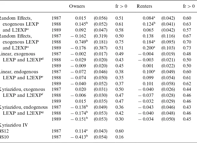
For the random e!ects and "xed e!ects panel data models (see also next subsection) we present for each wave implied elasticities of housing expenditure with respect to total expenditure (conditional on the ownership decision) in Table 5. We present means of these elasticities for owners and renters separately, weighted with housing expenditure. These can be interpreted as aggregate elasticities (see Banks et al., 1994).12Apart from the means and their standard errors, we also present the fraction of households for which the elasticity estimate is larger than zero.13In the pooled random e!ects models with LEXP and L2EXP assumed to be exogenous, the elasticities are positive but much smaller than one, suggesting that housing is a necessity. The standard errors, however, are sometimes quite large, yielding means which are insigni"cantly di!erent from zero. If LEXP and L2EXP are allowed to be endogenous, the elasticities are sometimes negative, though never signi"cantly so.
3.2. Fixed ewects
Using simultaneously more than one wave for estimation requires that we explicitly include the time period in the notation. As in the previous model, we decompose x
it intoxait, containing log total expenditure and its square, xbit,
containing log household income and its square, andx
dit, containing the prices
and taste shifters. Exclusion restrictions again yieldx
cit as a subvector of xdit.
The selection equation containsx
bitandxdit, while the budget share equations
containx
aitandxcit. The household speci"c e!ects will be (formally) treated as
time-invariant nuisance parameters, which, therefore, allows for correlation between "xed e!ects and regressors and errors. Throughout, we shall allow
Table 5
Housing expenditure elasticities for the panel data models (standard errors in parentheses)
Owners fr'0 Renters fr'0
Random E!ects, 1987 0.015 (0.056) 0.51 0.084! (0.042) 0.60 exogenous LEXP 1988 0.145" (0.052) 0.61 0.124" (0.041) 0.63
and L2EXP# 1989 0.092 (0.047) 0.58 0.065 (0.042) 0.57
Random E!ects, 1987 !0.162 (0.319) 0.50 0.138 (0.116) 0.67 exogenous LEXP 1988 0.749" (0.181) 0.75 0.184! (0.095) 0.70
and L2EXP# 1989 !0.176 (0.387) 0.51 0.200! (0.103) 0.73
Linear, exogenous 1987 !0.002 (0.017) 0.49 !0.004 (0.019) 0.48 LEXP and L2EXP$ 1988 !0.029 (0.020) 0.43 !0.003 (0.021) 0.50
1989 !0.009 (0.020) 0.45 0.001 (0.022) 0.50
Linear, endogenous 1987 !0.072 (0.046) 0.38 0.100! (0.049) 0.60 LEXP and L2EXP% 1988 !0.074 (0.050) 0.35 0.099 (0.054) 0.61
1989 !0.040 (0.052) 0.37 0.101 (0.058) 0.62
Kyriazidou, exogenous 1987 0.020 (0.031) 0.50 !0.040 (0.026) 0.44 LEXP and L2EXP& 1988 !0.006 (0.030) 0.47 !0.037 (0.028) 0.46 1989 0.015 (0.035) 0.47 !0.032 (0.029) 0.46 Kyriazidou, endogenous 1987 !0.138" (0.049) 0.36 !0.043 (0.046) 0.43 LEXP and L2EXP' 1988 !0.174" (0.053) 0.42 !0.040 (0.048) 0.46 1989 !0.151" (0.053) 0.30 !0.034 (0.050) 0.45 Kyriazidou IV
BS12 1987 0.114! (0.043) 0.60
BS10 1987 !0.413" (0.054) 0.16
!Signi"cant at the 5% level.
"Signi"cant at the 1% level.
#Based upon separate estimates for each wave (top panel Table 4).
$Based upon the estimates in the fourth column of Table 3.
%Based upon the estimates in the"fth column of Table 3.
&Based upon the estimates in the fourth column of the bottom panel of Table 4.
'Based upon the estimates in the"fth column of the bottom panel of Table 4.
x
ait to be endogenous. Estimation can be based on taking di!erences between
periodstandq,tOq. This yields, for households withd it"diq, y
pit!ypiq"b@pa(xait!xaiq)#b@pc(xcit!xciq)#(epit!epiq)
ifd
it"diq"p, p"0, 1
with
d
is"1(n@bxbis#n@dxdis#gi!uis*0), s"t,q.
Thus, ifd
it"diq"p,p"0, 1, we can write y
pit!ypiq"b@pa(xait!xaiq)#b@pc(xcit!xciq)#gptq(xbit,xbiq,xdit,xdiq)#e8pitq,
where the functionsg
ptq,p"0, 1, are given by
g
ptq(xbit,xbiq,xdit,xdiq)"EMepit!epiqDxbit,xbiq,xdit,xdiq,dit"diq"pN
and wheree8
pitq satis"es
EMe8
pitqDxbit,xbiq,xdit,xdiq,dit"diq"pN"0, p"0, 1.
The assumptions with respect to the error terms (e0it,e1it,u
it) determine the
functionsg
0tq andg1tq and the way to estimate the parameters. We discuss the
two that will be applied.
3.2.1. Linear panel data model
If we assume that no selection bias is present after di!erencing, i.e.,
g
ptq,0,p"0, 1, standard panel data estimation procedures can be used. In this
case there is no reason to estimate the auxiliary selection equation. Only the budget share equations need to be estimated. This corresponds to the assump-tion thatg
i!uitis independent ofe0itande1it, for allt, implying that possible
selection e!ects on the budget share equations only enter through correlation betweena
iand (gi,ui1,2,uiT). This assumption is often used in applications. An
example is the study of Pedersen et al. (1990) of wage di!erentials between public and private sector.
Estimation results for the linear "xed e!ects estimator are included in Table 3, both under the assumption that LEXP and L2EXP are exogenous (OLS), and allowing for their endogeneity (IV). A Hausman-type test compar-ing these two leads to rejectcompar-ing exogeneity for renters but not for owners. The wave dummies are always insigni"cant. The other variables (except AGE for owners) are always signi"cant. The estimated parameters of the variables LEXP and L2EXP imply a negative e!ect, ceteris paribus. The price e!ects are signi"cantly positive around 0.06, implying price elasti-cities of about !0.7 for both renters and owners. These elasticities are now not only conditional upon the exogenous variables and the choice between renting and owning, but also on the household speci"c "xed e!ects.
The same applies to the elasticities of housing expenditure with respect to total expenditure. They can be calculated in the same way as in the random e!ects panel data model. The aggregate elasticities for each panel wave are presented in Table 5. For owners the aggregate elasticities are insigni"cantly negative. For renters the elasticities are positive but small when allowing for endogeneity for LEXP and L2EXP, and signi"cant only for the 1987 wave. Comparing the results with those for the random e!ects model, the fairly large standard errors do not allow general conclusions concerning di!erences in sign or magnitude.
3.2.2. Semi-parametric model
For a panel with two time periods Kyriazidou (1997) proposes an estimator requiring weaker assumptions than those in the model discussed above. Her main assumption is exchangeability of the error terms. For the share equation of owners, this means that, conditional on (x
bit, xdit), all t, gi, a0*, and a1*, the vectors with error terms (e
1it, e1iq, uit, uiq) and (e1iq,e1it, uiq,uit) are identically
distributed. It implies that for households for which d
it"diq and n@
bxbit#n@dxdit"n@bxbiq#n@dxdiq, the e!ect of selection on the budget share
equation (i.e., theg-functions) is the same in periodstandq. For such observa-tions, di!erencing will not only eliminate the"xed e!ect, but also the selection e!ect. Note the di!erence with the linear model introduced above, where we could use all the observations, since the assumptions implied that correction terms were zero. Now, we only use that the correction terms are the same for certain observations. The subsample consisting of these observations is used for estimation.
Since observations with n@
bxbit#n@dxdit"n@bxbiq#n@dxdiq are scarce, all
observations for which the di!erence between these two values is su$ciently close to zero are used. This leads to weighted IV or weighted LS estimators for (b@
0a,b@0c)@ and (b@1a,b@1c)@. We present the IV estimation procedure for
the owners' share equation; the procedure applied to the other cases is very similar.
Denote the regressors in the budget share equations byx8
it"(x@ait,x@cit)@, and
a kernel with bandwidth satisfyings
1nP0 asnPR. Then the IV estimator for
(b@
1a,b@1c)@isSK~1wx SKwy1. The estimator is asymptotically normal with an
asymp-totic bias and an asympasymp-totic covariance matrix that can be estimated consis-tently, see Kyriazidou (1997, Theorems 1 and 2). The rate of convergence is (ns
1n)1@2.
We use the standard normal density function for the kernel. For choosing the bandwidth, we use the plug-in procedure given by Horowitz (1992): "rst, some initial value for the bandwidth is chosen and the parameter estimates, the estimate of the asymptotic bias, and the estimate of the covariance matrix are
14Details on this procedure are available upon request from the authors. We also experimented with various di!erent smoothness parameters, in particular, in case of the tests we employ (see remainder of this section). It turns out that in most cases the conclusions do not really di!er, although in a few cases, where the test results are close to the corresponding critical value, the conclusions change.
computed. These estimates are used to compute the MSE minimizing band-width, and then the bias and the covariance matrix are re-estimated.14
The approach for two time periods can easily be generalized to the case of more than two time periods. Given some estimates for the selection equation, the budget share equations can be estimated using the IV approach for each combination of panel waves (t,q). Minimum distance, preferably with the opti-mal weighting matrix, can then be applied to combine these estimates. Details can be found in Appendix D. To estimate the optimal weighting matrix, an estimate for the covariance matrix of the estimators for the di!erent time periods is required. These covariances converge to zero due to the fact that the band-width tends to zero. The proof is similar to that in Charlier (1994) and is included in Appendix D. The minimum distance estimator is, therefore, a weighted average of the estimators for each pair (t,q), (tOq), with weights given by the inverse of the corresponding covariance matrix estimate.
The above estimator requires a"rst-stage estimator (n(@
b,n(@d)@for (n@b,n@d)@. This
can be, for instance, smoothed maximum score (see Charlier et al., 1995, or Kyriazidou, 1997) or conditional logit, depending on the distributional assump-tions for the selection equation. Kyriazidou proposes to use smoothed max-imum score. Both estimators only use transitions from owning to renting and from renting to owning. Such transitions are scarce in our data, however. Consequently, it is impossible to estimate a very#exible speci"cation. Therefore, we will impose the stronger assumptions that the u
it(t"1,2,¹) are iid with
a logistic distribution, and use the conditional logit ML estimator to estimate the selection part of the model (see Chamberlain, 1980). Since this estimator for (n(@
b,n(@d)@ converges at a faster rate than those for (b@1a,b@1c)@ and (b@0a,b@0c)@, the
former will not a!ect the limit distribution of the latter. This is similar to the result in Kyriazidou (1997).
In order to retain as many observations as possible, we extend the conditional logit estimator to the case of unbalanced panels. Let c
i"(ci1,2,cit) denote
a vector of zeros and ones, with c
it"1 indicating that all the variables are
observed for household i in time period t. Assuming independence between
y
iandciconditional onxi, it is easy to show thatcican be treated as exogenous.
The conditional likelihood contribution of an observation then only depends on observed values of (y
it,xit).
We estimate the selection equation using the unbalanced panel for the years 1987}1989, consisting of 3917 households, with 2324 present in all three years,
15Since total expenditure does not play a role in the selection equation, observations with missing information on total expenditure are also used.
16See, for instance, Englehardt (1994), and Haurin et al. (1996). We thank the anonymous referee for pointing this out to us.
17Results in Appendix B show that most parameters tend to change slightly but not signi"cantly with the di!erent de"nitions for housing expenditure for owners.
953 in two years, and 640 in only one year.15This leads to 3063, 3274 and 3181 observations in the three waves. Important for the precision of the estimates, however, is the number of households that switch at least once between the two states renting and owning. This number is 168.
In the "xed e!ects logit model, only the coe$cients corresponding to the time-varying regressors are identi"ed. This implies that, due to little or no time variation in these variables, the constant term and the parameters of the education dummies, the dummy for being married, and the regional dummies cannot be estimated. Only the log price ratio (LRELPR), AGE, AGE2, LINC, L2INC and NCH remain. We added time dummies for each wave, two of which can be estimated; the coe$cient for the dummy for 1989 is normalized to zero.
The results of the selection equation are included in the"nal column of Table 2. The estimates for the time dummies show that the ownership rate increases over time, ceteris paribus. The age variables imply an inversely U-shaped pattern of the probability of owning similar to the other results in Table 2. LINC and L2INC are jointly insigni"cant. When L2INC is excluded, LINC remains insigni"cant. This result is di!erent from that for the random e!ect panel data model, where income had a signi"cant impact on the probability of home ownership. That"nding was probably due to the relation between permanent income and home ownership. In the "xed e!ects model, permanent income is part of the "xed e!ect, and the interpretation of our result is that transitory income components do not a!ect the home ownership decision signi"cantly. Regarding the home-ownership decision, generally housing theorists would expect a positive relationship between the probability of owning and transitory income. One possible reason for this is that mortgage lender imposed down-payment constraints prohibit ownership for some low wealth households. Positive transitory income could then be used to overcome the downpayment constraint, resulting in a positive relationship.16In the Dutch situation, such an e!ect does not seem to be present: in the Netherlands mortgage lenders generally do not impose downpayment restrictions; instead, they base their mortgage decisions mainly on (their estimate of ) the permanent part of the borrower's income.
The results on the budget share equations are included in the lower panel of Table 4.17The bias in the"rst step Kyriazidou estimates (see Kyriazidou, 1997,
Theorem 1) was generally large for AGE, AGE2, LOP and LRP, while it was small for the time dummy, LEXP and L2EXP ($9% of the parameter esti-mates) using 87/88 or 88/89 in estimation. However, the bias for these para-meters was much larger for 87/89 ($35%). The parameters related to AGE, AGE2, LEXP, L2EXP, and the prices are substantially di!erent from their random e!ects counterparts based on IV. The price e!ects remain positive, but are always insigni"cant. This implies that price elasticities are not signi"cantly di!erent from!1. Their point estimates are very close to!1 for owners, and
!0.8 (&OLS'estimates) or!0.9 (IV estimates) for renters.
The coe$cients of LEXP and L2EXP are strongly signi"cant. They imply that, ceteris paribus, the budget share spent on housing responds negatively to a change in total expenditure. The age e!ect is signi"cant for owners in case of IV, and for renters for &OLS'. In both cases the pattern is inversely U-shaped, with a maximum at age 35 and 54 for renters and owners, respectively.
To test for exogeneity of LEXP and L2EXP, we compare the Kyriazidou estimates using a Hausman test. Since the covariance between the estimators tends to zero asymptotically (see Appendix D), this test is easy to perform. The resulting chi-square test statistic is 10.31 for owners and 2.23 for renters. Both are smaller than the critical value of thes27at the 5% signi"cance level. Hence, the null of exogeneity of LEXP and L2EXP cannot be rejected.
To test the assumption of no selectivity bias in the linear panel data model, we perform a Hausman-type test comparing the IV parameter estimates in Tables 3 and 4. Because the Kyriazidou estimator converges slower than the linear panel data estimator, the limit distribution of the di!erence between the estimators is determined by the limit distribution of the Kyriazidou estimator only. The resulting values for the test statistics are 88.2 for owners and 23.7 for renters. Both are larger than the critical value of thes27 at any conventional signi"cance level. This indicates that the model that does not allow for correla-tion between the error terms in the share equacorrela-tions and the error term or"xed e!ect in the selection equation is misspeci"ed.
To test the assumption of no correlation between the household speci"c e!ects and (x@
bi,x@di)@ we perform a Hausman-type test based on the di!erence
between the Newey IV and the Kyriazidou IV estimates for those explanatory variables present in both estimates (AGE, AGE2, LEXP, L2EXP, and LOP or LRP). The limit distribution of the di!erence between the estimators is again determined by the limit distribution of the Kyriazidou estimator only. The resulting values for the test statistics are at least 232.1 for owners and at least 37.8 for renters. These exceed the criticals25 value at any conventional signi" -cance level, indicating that the random e!ects panel data model that does not allow for correlation between the household speci"c e!ects and the explanatory variables is misspeci"ed. This result continues to hold when we compare the estimates for owners and renters simultaneously.
18We used the balanced panel. Due to the extra time lag in the instruments we can only compute the estimates for the 1988 and 1989 waves of the panel so no minimum distance step is required.
19The elasticity estimates for the other models are much less sensitive to the de"nition of expenditures for owners (results not presented).
To test whether the coe$cients of the common variables in the budget share equation for owners and renters are the same we use a Wald test. Because¹"3, no household can both own a house for two periods or more and rent a house for two periods or more. As a consequence, the covariance between the estimates forb0andb1in Table 4 is zero, which makes it straightforward to perform the Wald test. The value of the test statistic is 11.74 which is below the 5% critical value of thes26distribution. This implies that we cannot reject the hypothesis that the coe$cients for the common variables are the same.
In Table 5 we include the weighted elasticity estimates for the Kyriazidou model, i.e., the aggregate elasticities of housing expenditure with respect to total expenditure. For owners the results are negative and insigni"cant under exogeneity of LEXP and L2EXP, and become signi"cantly negative when LEXP and L2EXP are endogenous. For renters the elasticity estimates are mostly negative and insigni"cant; only the 1987-wave results under exogeneity shows signi"cantly negative e!ect.
Again, the importance of the "xed e!ects for the interpretation of these results should be emphasized. Permanent income e!ects enter through the
"xed e!ect. The negative elasticities condition on these "xed e!ects, and, therefore, say nothing about the e!ects of permanent income. The negative estimates imply that transitory shocks on total expenditure tend to be negatively correlated to changes in housing expenditure. We have no economic explana-tion for this.
Under endogeneity, the signi"cant elasticities for owners thus seem to have the wrong sign. To see whether this is due to an inappropriate choice of instruments, we also replaced the instruments by the lagged values of log(household income) and its square.18The parameter estimates change: the elasticity estimate equals 0.006 with standard error 0.38; thus, it is insigni"cant with a much higher standard error than those reported in Table 5. The choice of current income variables as instruments, therefore, could explain the negative sign for the elasticities.
The "nal panel of Table 5 contains the estimates for the elasticities when di!erent measures of housing expenditure for owners are used (see Appendix B). The elasticities appear to be sensitive to the chosen measure.19
Since the Kyriazidou-model can be seen as our "nal model, we performed a speci"cation test on this model. A natural approach here is to perform a test on overidentifying restrictions in the minimum distance step. The realizations of the
20There are 7 parameters to be estimated. Using one pair of waves, only the di!erence of the two corresponding time dummies is identi"ed. Therefore we have 5]3#3"18 constraints in the minimum distance step. This yields 18!7"11 degrees of freedom.
test statistics are 41.50 for renters and 20.77 for owners, which both exceed the v211 critical value distribution at the 5% level.20
4. Conclusions
We have modelled expenditure on housing for owners and renters using endogenous switching regression models for panel data. In choosing the model assumptions we were guided by economic theory, but to a large extent also by the availability of suitable estimators and the nature of the data. We extended the standard switching regression model in several directions. We used (unbal-anced) panel data instead of cross-section data, and considered random e!ects and"xed e!ects models. For the random e!ects case, cross-section models and data can be used to obtain consistent estimates, but the "xed e!ects models require di!erent techniques. We used two of them, allowing for di!erent types of selection e!ects. Where possible, we tried to avoid normality assumptions and relied on semiparametric techniques. Finally, we focused on estimation tech-niques which allow some of the explanatory variables in the budget share equations to be endogenous.
The sample we used consists of three waves of the Dutch Socio-Economic Panel, combined with constant-quality prices, varying over time and space. We estimated the slope coe$cients in the random e!ects model using the cross-section data for each wave in a semiparametric model. We have compared results which do and do not take account of potential endogeneity of the variables related to total expenditure. Di!erences between these two sets of estimates mainly concern the parameter estimates related to the total expendi-ture variables themselves.
For the"xed e!ects panel data case we estimated two models. The"rst one is the linear panel data model which can be estimated using standard techniques. The alternative estimator based on weaker assumptions was proposed by Kyriazidou (1997). Here we estimated the parameters in the selection equation using conditional logit. The parameters in the budget share equations are estimated in a second step, making use of the conditional logit estimates. The models were compared using Hausman-type tests. The results indicate that both the random e!ects and the linear panel data model are too restrictive. Exogene-ity of total expenditure variables is not always rejected. Finally, we also applied a test on overidentifying restrictions in the Kyriazidou (1997) model, the most
general model that we considered. The results suggest that even the #exible Kyriazidou (1997) model is misspeci"ed.
Our overall conclusion is that standard models with random e!ects which can be estimated with cross-section data, and linear panel data models which only allow for very speci"c selection mechanisms, are rejected against the #exible semi-parametric"xed e!ects model of Kyriazidou (1997). The various models also lead to diverging conclusions on the elasticities of interest. The price elasticities for renters and owners (conditional on the choice between owning and renting and taste shifters and income) are about!0.5 in the random e!ects models, but are closer to!1 (owners) or !0.8 (renters) in the "xed e!ects models. Compared to the estimates in the literature for the UK and the US, the latter are somewhat large. The estimates of total expenditure elasticities vary from signi"cantly positive in the random e!ects models to insigni"cantly (ren-ters) or even signi"cantly (owners) negative in the most general "xed e!ects model, though the latter result for owners is sensitive to the way in which housing expenditures for owners are de"ned. Part of the di!erence can be explained by a positive impact of permanent income on housing demand, an e!ect which is controlled for in the "xed e!ects model but not in the random e!ects model. The estimated total expenditure elasticities are quite low compared to estimates of income elasticities in the literature. This comparison may not be valid, however, since the elasticities in the literature are de"ned di!erently and, for example, typically do not condition on the choice between renting and owning.
Acknowledgements
We thank two anonymous referees, Marno Verbeek and seminar participants at Rice University for helpful comments. Research of the third author was possible due to a fellowship of the Netherlands Royal Academy of Arts and Sciences (KNAW). We are grateful to Statistics Netherlands (CBS) for providing the data.
Appendix A. Data appendix
In this appendix we give some details on the construction of the variables for 1987}1989, used in the application. For 1989, macro-data are available which will be compared to our data.
A.1. Housing
Initial dataset: 3613, 3818, 3896 households for 1987, 1988 and 1989, respec-tively.
Dropped from the analysis are:
f families that live for free ($0.8%);
f families with a total income below D#. 1,- per month ($200 obs);
f families that receive a so-called huurgewenningsbijdrage (i.e., a governmental
allowance for people who experienced a large rent increase because of renova-tion of their dwelling or who had to search for a di!erent dwelling after pull down of their previously rented dwelling). The reason for this latter drop is that the amount is a substantial part of the housing expenditure (16% on average) and it is not clear from the data whether this amount is included in the answers on rent payments or not ($1.2% of the renters).
A.2. Housing consumption for owners
(1!tax) erfpacht#tax huurwaardeforfait#(1!tax) interest payment#
foregone interest!increase in the value of the house#maintenance costs#
eigenaarsgedeelte onroerend goedbelasting#opstalverzekering.
Here erfpacht is the amount of money you have to pay if you do not own the land on which your dwelling is built (which is partly deductible), tax is the marginal tax rate of the most earning adult in the household, huurwaardeforfait is tax levied on the value of the house of owners, eigenaarsgedeelte onroerend goedbelasting is municipal tax for house owners and opstalverzekering is a house insurance for "re, broken windows etc. Expenditure on gas/water/ electricity/heating is excluded.
A.3. Computation of thevariables in expenditure for owners
Approximately 140 house owning families dropped out because the value of the house is not known, which is necessary to correct for, among other things, huurwaardeforfait. In the data we have either the amount spent on interest payments on the mortgage or the interest rate on the mortgage. If we only have the interest rate on the mortgage we computed the interest payments by multiplying this percentage with the mortgage value. If the mortgage value is not reported we used 149,000, 155,000 and 163,000 (the average value of a house for 1987, 1988 and 1989). The numbers of observations a!ected are 22, 27 and 22, respectively. Foregone interest is set equal to 0.04 times the di!erence in the value of the house and the mortgage value. Maintenance costs are de"ned as 2% of the value of the house. In the main text we investigate the sensitivity of the results with respect to the percentage increase in the value of a house and the percentage used in the maintenance costs. Because the eigenaarsgedeelte on-roerend goedbelasting can di!er per municipal it is calculated as follows: we have data over 1986}1989 on Tilburg and we will consider Tilburg to be representative for its province. Per province we have the amount of tax that was
paid to the local government per inhabitant of the municipality (CBS, 1987, Statistiek der gemeentebegroting). The eigenaarsgedeelte onroerend goedbelast-ing per province is calculated as the"gure for Tilburg times the relative tax per inhabitant of the province. The relative tax for the provinces is approximately constant over time. The opstalverzekering is simply 12.95 times the value of the house divided by 100,000 (Budgethandboek NIBUD, 1987).
A.4. Computation of marginal tax rate
In the SEP we only observe net income like net wages, net unemployment bene"ts, net pensions, etc. To calculate the marginal tax rate we need gross income of the spouse that earns most because he/she will have to report the tax related issues of owning a house (like e.g. huurwaardeforfait). From the net income we could try to invert the tax system and infer gross income. However, this is a very cumbersome approach. Therefore, we will follow Euwals and van Soest (1999). Gross income is already available for individuals with a paid job. We now estimate a net wage equation using the households in which at least one individual has a paid job. An important variable to be included is the tax free allowance (TFA). Constructing this for married couples involves the gross income of the other spouse. All the households for whom we could determine the TFA were included in estimation. The equation estimated is the same as in Euwals and van Soest (1999), i.e. without a constant term. Without making di!erences between men and women we got anR2of 0.9955 and the parameter estimates are fairly similar. Given the net income we can now estimate gross income by inverting the relationship. By taking derivatives of net income with respect to gross income we can estimate the marginal tax rate.
A.5. After tax constant quality prices of housing
In the budget share equations, after tax constant quality prices of housing are used. After tax prices are used to take into account tax deduction of housing for owners and hence tax e!ects are only relevant for owners. Constant quality prices of housing for both renters and owners are constructed as follows:
f De"ne regions and house-categories. For each combination of (renter, region,
house-category) and (owner, region, house-category) we determine the frac-tion of houses in it, based on our 1987 sample. We also determine the median rent (for renters) and the median house price (for owners), based on the sample for 1987, 1988 and 1989.
f Constant quality prices of housing are then computed by multiplying the
fraction for each combination with the median rent or median house price, respectively. The resulting constant quality prices of housing vary for renters and owners and by regions.
21The regions are the 12 Dutch provinces; however, Overijssel and Flevoland are grouped together because the latter is very small, yielding 11 regions.
22The"rst type consists of detached, semi-detached or corner houses and the second type consists of row houses and apartments.
To limit the number of combinations we distinguish 11 regions21 and two house categories.22 Together with the owners/renters distinction this results in 44 categories. To obtain the weights and prices the sample consists of about 2000 observations (the reduction is mainly due to the absence of information on house-category), so on average 45 observations are available for each cell. To reduce the in#uence of outliers the median rent and house price are used. For owners, the constant quality prices of housing are multi-plied by 1 minus the marginal tax rate for the household in the particular year.
A.6. General remarks concerning the data
The following data cleaning operations have been applied:
f People who got married or divorced are left out in the analysis to avoid
dependence between households in the sample ($140 households per year);
f Households that spend more than 0.6 times their monthly income on housing
($130 households per year) are also left out.
In general, we lose approximately 670 households per year. If we use only the observations with income budget shares smaller than 0.6 we end up with 2936, 3157 and 3261 observations.
A.7. Comparing the data with macro-data
We will compare the 1989 with the "gures in Woningbehoeftenonderzoek 1989/1990 reported by Statistics Netherlands (CBS). Their de"nitions for rent and income are the same as the ones we use. For renters the CBS tabulates rent, net annual income and budget shares. The de"nition of expenditure on housing for owners di!ers from our measure. The CBS measure of housing expenditure includes expenditure on the mortgage, erfpacht, opstalverz., eigenaarsgedeelte onroerend goed belasting, rijksbijdrage eigen woning bezit and tax issues like interest, erfpacht, huurwaardeforfait en rijksbijdrage eigen woning bezit. We constructed this measure without opstalverz., eigenaarsgedeelte onroerend goed belasting, rijksbijdrage eigen woning bezit and related tax issues. For owners the CBS tabulates net yearly income and budget shares.
Comparing the 1989 data with the statistics in the Woningbehoeftenonder-zoek 1989/1990 we conclude that:
f House owners are overrepresented in our sample. We see two reasons for this:
the group of one-person households is underrepresented and 75% of this group rents, and the owners are overrepresented in the more-than-one-person households.
f For renters our rent data follow the results of the CBS, but low income
households ((26,000 net per year) are underrepresented. Furthermore, the higher budget shares are overrepresented yielding an average budget share of 0.20 instead of 0.18.
f The distribution of net annual income for owners with a mortgage has higher
fractions in the higher income brackets. The distribution of budget shares has the same property and the average budget share is 0.148 instead of 0.137.
f Households owning a house without a mortgage are underrepresented.
In general the data have the following features:
f the density of income shifts a little bit to the right over time;
f the density of the budget shares for renters remains approximately the same
over time;
f the density of the budget shares for owners is slightly shifted to the right when
compared to the 1989 macro-data;
f the density of the interest payments on mortgages looks the same for all years.
However, the average value is increasing (slightly) over 1987}1989.
Although the 1986 data are not used in the main text, we also compared them to the macro-data for 1986. The results are similar to those for 1989.
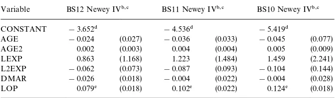
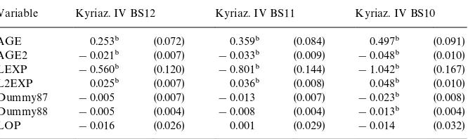
Appendix B
In this appendix we will investigate the sensitivity of the cross-section Newey IV results for 1987 and the panel data Kyriazidou IV results with respect to the maintenance costs and the mortgage costs in housing consumption for owners. Let BS1ab denote the budget share spent on housing for owners with a% increase of the value of a house (a"0, 1, 2, 3, 4) and b% of the value of the house as the maintenance costs (b"1, 2). In the main text a equals 1 and
b equals 2. From the de"nition of housing costs for owners it follows that BS1ab"BS1a#1,b#1 so, for example, BS121"BS132. Because the aver-ages for BS142, BS132 (and hence BS131 and BS121) are very low compared to the average for renters we only consider BS122, BS112 and BS102. The last digit can then be dropped, because it is"xed at 2, so that we write BS1a,a"2, 1, 0. Thus, BS11 is used throughout the main text. The means for BS12, BS11 and BS10 are, respectively, 0.15, 0.20 and 0.24 with standard errors of 0.08, 0.09 and 0.11.