Economics Letters 69 (2000) 123–128
www.elsevier.com / locate / econbase
The first-order stochastic dominance ordering of the
Singh–Maddala distribution
*
Stefan Klonner
¨ ¨
Sudasien Institut der Universitat Heidelberg, INF 330, 69120 Heidelberg, Germany
Received 3 June 1999; accepted 3 March 2000
Abstract
Given two distributions from the Singh–Maddala family, this paper investigates how to determine whether one distribution first-order stochastically dominates the other. The resulting criteria are also applied to the Dagum type I family of distributions. 2000 Elsevier Science S.A. All rights reserved.
Keywords: Ranking income distributions; Singh–Maddala distribution; Inequality; Social welfare
JEL classification: C49; D31; D63
1. Introduction
The family of distributions proposed by Singh and Maddala (1976) has been a popular model for describing the distribution of income or consumption expenditure (see McDonald, 1984; Brachmann et al., 1996). The cumulative distribution function (cdf) is given by
a 2q
F(x; a, b, q)512[11(x /b) ] . (1)
In empirical applications, the parameters b, a and q are estimated to facilitate intertemporal or international comparisons of income distributions with a view to drawing conclusions about inequality and social welfare. Where inequality is concerned, comparisons are usually made using the
Lorenz-¨
ordering. For the Singh–Maddala family, Wilfling and Kramer (1993) have derived necessary and sufficient conditions to determine the Lorenz-ordering of two distributions in terms of the parameters
a and q. Since it is mean-free, however, the Lorenz-ordering does not provide an answer to the
question which one of two distributions implies higher social welfare. If we focus on the subclass of
*Tel.:16-221-548-754; fax: 16-221-545-596.
E-mail address: [email protected] (S. Klonner).
additively separable welfare functions satisfying monotonicity in each individual’s income, then a comparison with respect to social welfare will be equivalent to a comparison of the associated cdf’s with respect to first-order stochastic dominance (FSD). Moreover, FSD implies higher order stochastic dominance as well as generalized Lorenz-dominance (see Cowell, forthcoming) which is a central
1
concept for comparing income distributions in many fields of economics.
Distribution G is said to (weakly) first-order stochastically dominate H if, and only if, G(x)#H(x)
for all x (see Cowell, forthcoming). Although some distribution-free tests for FSD have been developed (see Schmid and Trede, 1996, for a recent example), virtually no attempts have been made to address this issue in the context of parametric distributions. This I shall attempt to do for the Singh–Maddala (SM) family.
As in the case of the Lorenz-ordering, the FSD ordering of distributions from the Singh–Maddala family is not complete, i.e. in many cases the cdf’s will intersect. Moreover, while for the Lorenz-ordering the scale parameter b plays no role, the FSD ordering will depend on all three parameters, rendering it impossible to give a set of closed form ‘if, and only if’ conditions.
2. Necessary and sufficient conditions for first-order stochastic dominance
Theorem 1 gives necessary conditions for first-order stochastic dominance.
Theorem 1. Let F and F be SM distribution functions, with parameters a , b and q (i1 2 i i i 51, 2),
respectively. If F first-order stochastically dominates F , then
1 2
(a) a1$a and2
(b) a q1 1#a q .2 2
t
Proof. Define the family of strictly increasing functions u (x)5x /t, t±0 and the corresponding family
t
of additively separable social welfare functions W (F )t 5e u (x) dF(x)t 5mt(F ) /t, wheremt(F ) denotes the tth moment associated with F. We further need the following representation of the tth moment of the SM family obtained by McDonald (1984):
t
mt(F )5bG(11t /a)G( q2t /a) /G( q) (2)
where G(?) denotes the complete gamma function.
(a) Assume that a1,a and let t approach2 2a from above. In this case, 11 s 1t /a1d will approach zero. Inspection of (2) and recalling that limz→0 G(z)5 ` reveals that this implies that W (F ) willt 1
approach minus infinity, while W (F ) will approach a finite negative number. Thus for somet 2
t9 . 2a we have W (F )1 t9 1 ,W (F ). Since F (x)t9 2 1 #F (x) for all x implies W (F )2 t 1 $W (F ) for all t (seet 2
Saposnik, 1981), W (F ),t9 1 W (F ) contradicts Ft9 2 1#F .2
(b) Assume that a q1 1.a q and let t approach a q from below. Now the term2 2 2 2 G( q22t /a ) and2
thus W (F ) will approach plus infinity, while W (F ) will approach a finite positive number. Thus fort 2 t 1 some t*,a q we have W (F )2 2 t * 1 ,W (F ), which contradicts Ft * 2 1#F .2 QED
1
S. Klonner / Economics Letters 69 (2000) 123 –128 125
It is interesting to note that the necessary conditions given in Theorem 1 are in direct contrast to ¨
those for Lorenz-dominance obtained by Wilfling and Kramer (1993) who showed that F Lorenz-1 dominates F if, and only if, a2 1$a2 and a q1 1$a q . Thus, if two distributions can be Lorenz-2 2
ordered, there will be no ordering according to FSD and vice versa. This is a serious drawback of the SM family since, in general, a distribution G can first-order and Lorenz-dominate a distribution H at the same time.
We state an inequality for sums introduced by Pringsheim (1902a,b, see also Hardy et al., 1952, Theorem 19) that will be needed for the proof of Theorem 2:
n r 1 / r n p1 / p
Lemma 1. For positive r, p and c , k51, . . . , n,
s
o cd
#s
o cd
if, and only if, r$p.k k51 k k51 k
A set of sufficient conditions for first-order stochastic dominance is set out in:
Theorem 2. If a1$a , a q2 1 1#a q and b2 2 1$b , then F2 1 first-order stochastically dominates F .2
The next theorem covers the special cases where either (a) or (b) of Theorem 1 holds with equality and, as a third case, b1$b :2
for all positive z. Clearly, this inequality will hold for all z if, and only if, q /q is not bigger than1 2 unity and, for z50, the derivative of the left hand side is not bigger than the derivative of the right
1 / a
(c) Necessity follows from Theorem 1, sufficiency from Theorem 2. QED
S
.
Klonner
/
Economics
Letters
69
(2000
)
123
–
128
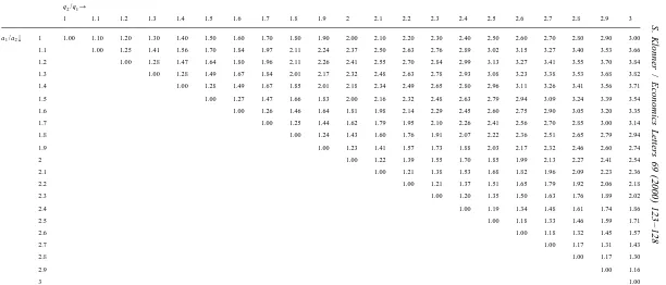
Table 1
Values of v(a /a , q /q )
1 2 2 1
q /q2 1→
1 1.1 1.2 1.3 1.4 1.5 1.6 1.7 1.8 1.9 2 2.1 2.2 2.3 2.4 2.5 2.6 2.7 2.8 2.9 3
a /a1 2↓ 1 1.00 1.10 1.20 1.30 1.40 1.50 1.60 1.70 1.80 1.90 2.00 2.10 2.20 2.30 2.40 2.50 2.60 2.70 2.80 2.90 3.00
1.1 1.00 1.25 1.41 1.56 1.70 1.84 1.97 2.11 2.24 2.37 2.50 2.63 2.76 2.89 3.02 3.15 3.27 3.40 3.53 3.66 1.2 1.00 1.28 1.47 1.64 1.80 1.96 2.11 2.26 2.41 2.55 2.70 2.84 2.99 3.13 3.27 3.41 3.55 3.70 3.84
1.3 1.00 1.28 1.49 1.67 1.84 2.01 2.17 2.32 2.48 2.63 2.78 2.93 3.08 3.23 3.38 3.53 3.68 3.82 1.4 1.00 1.28 1.49 1.67 1.85 2.01 2.18 2.34 2.49 2.65 2.80 2.96 3.11 3.26 3.41 3.56 3.71
1.5 1.00 1.27 1.47 1.66 1.83 2.00 2.16 2.32 2.48 2.63 2.79 2.94 3.09 3.24 3.39 3.54 1.6 1.00 1.26 1.46 1.64 1.81 1.98 2.14 2.29 2.45 2.60 2.75 2.90 3.05 3.20 3.35
1.7 1.00 1.25 1.44 1.62 1.79 1.95 2.10 2.26 2.41 2.56 2.70 2.85 3.00 3.14
1.8 1.00 1.24 1.43 1.60 1.76 1.91 2.07 2.22 2.36 2.51 2.65 2.79 2.94
1.9 1.00 1.23 1.41 1.57 1.73 1.88 2.03 2.17 2.32 2.46 2.60 2.74
2 1.00 1.22 1.39 1.55 1.70 1.85 1.99 2.13 2.27 2.41 2.54
2.1 1.00 1.21 1.38 1.53 1.68 1.82 1.96 2.09 2.23 2.36
2.2 1.00 1.21 1.37 1.51 1.65 1.79 1.92 2.06 2.18
2.3 1.00 1.20 1.35 1.50 1.63 1.76 1.89 2.02
2.4 1.00 1.19 1.34 1.48 1.61 1.74 1.86
2.5 1.00 1.18 1.33 1.46 1.59 1.71
2.6 1.00 1.18 1.32 1.45 1.57
2.7 1.00 1.17 1.31 1.43
2.8 1.00 1.17 1.30
2.9 1.00 1.16
S. Klonner / Economics Letters 69 (2000) 123 –128 127
distributions under comparison intersect or not, namely when conditions (a) and (b) of Theorem 1 both hold with strict inequality together with b2.b . Therefore I provide a table that, together with1
Theorem 1, fills this gap. First note that F1#F is equivalent to2
a2 a / a1 2 q / q1 2
(b /b )2 1 #z /
s
(11z ) 21d
(4)for all positive z. Further, the necessary conditions of Theorem 1 can be written as
1#a /a1 2#q /q .2 1 (5)
Table 1 therefore reports the minimum of the r.h.s. of (4) with respect to z,v(a /a , q /q ), for pairs
1 2 2 1
of a /a and q /q over a range that is sufficient for most applications and that satisfies (5). Thus, F1 2 2 1 1
a2
first-order stochastically dominates F if, and only if, (a) and (b) of Theorem 1 hold and (b /b )2 2 1 #
v(a /a , q /q ).
1 2 2 1
3. The dagum type I family
The cdf of the Dagum type I model (Dagum, 1977) is given by
˜ ˜ a2q
˜ ˜
˜ ˜
G(x; a, b, q )5
s
11(b /x)d
.A comparison of this with the SM family can be found in Kleiber (1996), who also obtained necessary and sufficient conditions for Lorenz-dominance.
Rearranging (3) together with a change of variable yields the following lemma.
˜
˜ ˜
Lemma 2. Let G and G be Dagum type I distribution functions with parameters a , b and q1 2 i i i
(i51,2), respectively, and define F(x; a, b, q) as in (1). Then G first-order stochastically dominates 1
˜ ˜
˜ ˜ ˜ ˜
G if, and only if, F(x; a , 1 /b , q ) first-order stochastically dominates F(x; a , 1 /b , q ).2 2 2 2 1 1 1
Thus all results obtained for the SM family in Section 2 can be applied to the Dagum type I family
˜
˜ ˜
if we replace a , b and q by a , 1 /b and q , respectively, and a , b and q correspondingly.1 1 1 2 2 2 2 2 2
Acknowledgements
I am indebted to Martin Biewen, Carsten Fink, Christian Kleiber, Ramona Schrepler and Bernd Wilfling for useful comments. Special thanks to Clive Bell for intensive ongoing discussions. The usual disclaimer applies.
References
Brachmann, K., Stich, A., Trede, M., 1996. Evaluating Parametric Income Distribution Models. Allgemeines Statistisches Archiv. 80, 285–298.
´ Dagum, C., 1977. A new model of personal income distribution: specification and estimation. Economie Appliquee 33,
327–367.
´
Hardy, G., Littlewood, J.E., Polya, G., 1952. Inequalities, 2nd Edition. Cambridge University Press, Cambridge. Kleiber, C., 1996. Dagum vs. Singh–Maddala income distributions. Economics Letters 53, 265–268.
Lambert, P., 1989. The Distribution and Redistribution of Income. Blackwell, London.
McDonald, J.B., 1984. Some generalized functions for the size distribution of income. Econometrica 52 (3), 647–663. ¨
Pringsheim, A., 1902a. Zur Theorie der Ganzen Transzendenten Funktionen. Munchner Sitzungsberichte 32, 163–192. ¨
Pringsheim, A., 1902b. Zur Theorie der Ganzen Transzendenten Funktionen. Munchner Sitzungsberichte 32, 295–304. Saposnik, R., 1981. Rank dominance in income distribution. Public Choice 36, 147–151.
Schmid, F., Trede, M., 1996. Testing for first-order stochastic dominance: a new distribution-free test. Statistician 45, 371–380.
Singh, S.K., Maddala, G.S., 1976. A function for size distribution of incomes. Econometrica 44, 963–970. ¨