www.elsevier.com / locate / econbase
Evaluating the semi-nonparametric Fourier, AIM, and neural
networks cost functions
a b c ,
*
Adrian R. Fleissig , Terry Kastens , Dek Terrell
a
Department of Economics, California State University–Fullerton, Fullerton, CA 92834-6848, USA
b
Department of Agricultural Economics, 304F Waters Hall, Kansas State University, Manhattan, KS 66506, USA
c
Department of Economics, 2114 CEBA, Baton Rouge, LA 70806, USA
Received 26 April 1999; accepted 14 December 1999
Abstract
This study compares how well three semi-nonparametric functions, the Fourier flexible form, asymptotically ideal model, and neural networks, approximate simulated production data. Results show that higher order series expansions better approximate the true technology for data sets that have little or no measurement error. For highly nonlinear technologies and much measurement error, lower order expansions may be appropriate.
2000 Elsevier Science S.A. All rights reserved.
Keywords: Semi-nonparametric; Fourier; AIM; Neural networks
JEL classification: C14; D12
1. Introduction
Semi-nonparametric (SNP) forms represent the latest development in a trend toward using functional forms that can globally asymptotically approximate more complex data generating functions, a property Gallant (1981) defines as Sobolev-flexibility. In applications, however, these
1
SNP functions can give different results and implications for policymakers and firms. Our goal is to evaluate the approximations of the SNP functions when the data have as much as 10 and 20% measurement error. Given data with considerable measurement error, it is possible for the SNP
*Corresponding author. Tel.: 11-225-388-3785; fax:11-225-388-3807.
E-mail address: [email protected] (D. Terrell)
1
For example, Fleissig et al. (1997) compare estimates of the elasticity of substitution between capital and labor for U.S. manufacturing using three SNP forms. They find that although all forms predict that capital and labor are substitutes in production, the magnitudes of elasticity estimates vary considerably across SNP forms.
functions to provide a poor approximation by fitting the ‘noise’ around the true data generating
2
process. Furthermore, SNP forms are also compared to two Diewert-flexible functional forms. While
3
previous studies compare one SNP function to parametric flexible forms, this paper provides the first comparison of how well three SNP functions, the Fourier flexible form, asymptotically ideal model (AIM) and neural networks (NN), approximate data generated from different technologies.
2. Semi-nonparametric forms
Economists must choose among various functional forms to approximate an unknown technology. In this study, we examine the ability of functional forms to approximate a unit cost function. Output is omitted which is equivalent to approximating a constant returns to scale cost function. Once the appropriate functional form is determined for the unit cost function, additional terms can be appended to address returns to scale.
2.1. The Fourier cost function
The Fourier approximation of the true cost function developed by Gallant (1982) is:
A J
xi5ln pi1ln a is a logarithmic transformation of prices. The constant a chosen so that x is strictlyi i i
25
positive ln ai5 2min(ln p )i 110 and the location shift does not affect the results. The scaling factor l is chosen a priori, l56 / max(x ), to ensure that all x are within the interval (0,2i i p) (see Gallant, 1982 for details). The sequence of multi-indices hkaj represents the partial derivatives of the Fourier cost function with each set producing a particular Fourier series expansion. The cost function
n n
is linearly homogeneous in price if oi51bi51 andoi51 kia50 and these restrictions are imposed in estimation. The Fourier cost share Eqs. are:
A J
Estimation requires selecting the order of the Fourier expansion which depends on A and J. For reliable asymptotics, Huber (1981) shows that the number of parameters required is about two-thirds the root of the effective sample size. With two Eqs. and 100 observations this amounts to estimating about 35 parameters. With A55 and J53, the Fourier has 37 parameters which are used in estimation. However, when the data are measured with error, higher order Fourier expansions may fit
2
Diewert (1974) defines a flexible form as any function that gives a local second order approximation to the data generating function.
3
the ‘noise’ around the true technology and it may be better to estimate a lower order expansion. To investigate this possibility, we also use the Chalfant and Gallant (1985) settings of A53 J51 (13 parameters) and A56 J51 (22 parameters).
2.2. The AIM cost function
¨
The Barnett and Jonas (1983) AIM model is defined on the basis of the Muntz–Szatz approximation of the cost function:
which is homogeneous of degree one in factor prices if the exponent sets sum to one. AIM is dense in the space of continuous functions if all uaj,1. Following Barnett et al. (1991), Terrell (1995) and Jensen (1997), we use the series 1 / 2, 1 / 4, 1 / 8, . . . to complete the definition of AIM. The resulting cost function is best understood by looking at the three input model at low orders:
AIM 1: Six parameters
It is apparent that AIM 1 is the generalized Leontief flexible functional form. AIM 2 includes all combinations of prices with exponents 1 / 4,1 / 2,3 / 4 summing to one and has AIM 1 as a special case.
m
At order m, AIM includes combinations of prices raised to the power (1 / 2) . The system of AIM input demands estimated are derived using Shephard’s lemma.
2.3. The neural network approximation of the cost function
4
The neural network (NN) approximation of a three-input cost function of a system of demand Eqs. is: NN(h): 7h13 parameters, 1 hidden layer
x( p)5f( f( pW11w )W1 21w )2
where, x is a 1 by 3 vector of input demands and p is the associated 1 x 3 input price vector. W , w ,1 1
W , and w , are matrices or vectors of parameters (weights) to be estimated. W is dimensioned 3 x h2 2 1
and w is 1 x h. For conformability, W and w must be h x 3 and 1 x 3, respectively. In general, w1 2 2 1
4
and w are analogous to the intercept in conventional econometric models. The number of nodes in2
this single-hidden-layer model is denoted by h, and must be determined empirically (we considered values of h51, 3, and 5). A larger h (more nodes in the hidden layer) implies a higher order
5
functional approximation. The function f, operating on its matrix argument on an element-by-element basis, is an arbitrary bounding function whose first derivative is typically a function of f. The function
f is often approximated by the sigmoid function f(x)51 /(11exp(2x)) with corresponding first
derivative, f9(x)5f(x)(12f(x)) and is used in this paper.
2.4. The translog
In addition to the SNP forms, we estimate two Diewert flexible forms, the generalized Leontief (which is equivalent to AIM1) and the following translog cost function:
C( y,P)5exp(h( y,P)) where h( y,P)5d01
O
d ln pi i1O O
gijln p ln pi ji i j
The parameters satisfy the restrictions of symmetry and linear homogeneity in prices oidi51,
gij5gji, and oigij50 and the input demands are derived using Shephard’s lemma.
3. Experimental design
The data used to evaluate the flexible forms are simulated from the CES and generalized Box–Cox functions. These data generating functions are used because they give substitution elasticities of the magnitudes often found in empirical applications. In addition, Terrell (1995) uses the CES function to evaluate the AIM whereas Chalfant and Gallant (1985) use the generalized Box–Cox technology to evaluate the Fourier. Therefore, by considering these technologies, it is unlikely that the SNP results are biased toward one functional form because of the choice of the data generating function.
The CES cost function and input demands used by Terrell (1995) to evaluate the AIM are:
n (r21 ) /r
r/ (r21 ) 1 / ( 12r) 1 / (r21 ) C( y,P)5y
S
O
piD
and xi5C( y,P) pii51
The generalized Box–Cox and input demands used by Chalfant and Gallant (1985) with symmetry and homogeneity imposed, are:
5
n n 1 /v
v/ 2 v/ 2 12v v/ 221 v/ 2 C( p)5
F
2 /vO O
uijPi PjG
and xi52 /vC PiO
uijPji51 j51 j
The elasticities are calculated using the Morishima elasticity of substitution:
pi pi
] ]
sij5Cij? 2Cii?
xj xi
because, as Blackorby and Russell (1989) show, the Allen–Uzawa measure is incorrect when there are more than two variables. Note that the Morishima elasticity is non-symmetric unless the data generating function is a member of the constant elasticity of substitution (CES) family. For the CES function, the Morishima elasticities of substitution are symmetric and constant whereas the generalized Box–Cox function yields variable non-symmetric Morishima elasticities.
The trivariate data generating process of Chalfant and Gallant (1985) is used to construct price series similar to those in the Berndt and Wood (1975) data set. Input prices are deflated by the price of output and then fitted by a first order autoregression ln Pt5b1e with et t5Ret211et giving
6
estimates of R andb, where the elements ofb correspond to capital, labor and other inputs. We then generate a set of 150 observations for each input price by combining normally distributed innovations with the estimates from the autoregression. The input demands with a corresponding wide range of Morsihima elasticities are generated from the CES and generalized Box–Cox forms using the parameter settings from Table 1 and price series.
Data with 10 and 20% measurement error are generated by adding normally distributed errors
2 2
N(0,s10%) and N(0,s20%) to the input demands. It is important to avoid choosing an unrealistically large or small innovation for the stochastic error component of the simulated data. We address this issue by setting the variance of the stochastic component to be a proportion (10 or 20%) of the variance of the nonstochastic of input demands. For example, a 10% error for input i requires setting
2
si,10%50.10?Var(x ), which ensures that approximately 90% of the variation of input i is attributablei
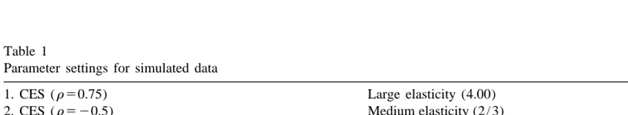
Table 1
Parameter settings for simulated data
1. CES (r 50.75) Large elasticity (4.00)
2. CES (r 5 20.5) Medium elasticity (2 / 3)
The Berndt–Wood data have capital, labor, energy, and materials. We construct a share-weighted aggregate of energy and materials inputs (defined as other inputs) to reduce the number of inputs to three. The estimate of b was (0.09761,
to variation in prices. This provides a total of 15 data sets which have either, no error, 10% error, or 20% error for each technology.
4. Results
7
We present the results using graphs, tables and response surface estimation. We focus on the average root mean square error (fitted values less true values) from each function across the three input demands and a similar average across the six Morishima elasticities. The CES data sets vary the elasticity of substitution between inputs from 0.2 to 4.0. The Box–Cox parameter settings correspond to design technologies 5 and 7 of Chalfant and Gallant (1985). By construction, all Box–Cox and CES parameter settings lead to technologies satisfying concavity, monotonicity, homogeneity and symmetry at every price used in the data set and at all forecast prices. Homogeneity and symmetry
8
constraints are imposed in the translog, AIM, and Fourier models. Given that the Fourier is estimated in shares, it may approximate the shares slightly better than the AIM and NN. For similar reasons, AIM and the NN may have an advantage in approximating input demands. Our analysis reveals that the results are very similar for the shares and input demands; thus we only report the results for the input demands. The functions are estimated using the first 100 observations, with the last 50 observations reserved for out-of-sample forecasts.
4.1. Basic results for simulated data
For each technology, we generated data with no error, 10% error, and 20% error. Not surprisingly all three SNP forms performed well for data generated with no error. Increasing the order of expansion led to a better approximation in all cases, though AIM and the Fourier series tended to provide a slightly better approximation than the neural networks for most technologies.
For data generated with error, fitting the observed data points does not guarantee an accurate approximation of the unknown technology. Thus, we evaluate how well the SNP functions approximate the true technology using data generated with 10 and 20% error. In most cases the results show that the SNP forms continue to better approximate the true data generating function than the translog but there is some evidence of overfitting by the SNP forms.
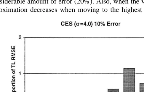
Fig. 1 graphs the average RMSE for all inputs from the SNP functions for the most nonlinear CES (s54) technology having 10% error, divided by the average RMSE for the translog. The approximation of the true technology improves for each SNP form by increasing the order of the expansion from AIM 1 to AIM 2, Fourier with J51, A53 to J51, A56 and a neural network with
7
Both the Fourier system of the cost function and the first two shares and the AIM system of three input demands are estimated using maximum likelihood estimation. The likelihood functions often proved quite flat, so convergence criteria were tightened and results were replicated with numerous starting values. Matlab Numeric Computation Software (Math Works Inc., Natick, Massachusetts, 1994) was used to perform the network estimations. For a more comprehensive description of the neural network functional form and the associated analytical derivatives for partial effects (Kastens et al., 1995).
8
Fig. 1. Ratio of RMSE to translog RMSE for input demands.
one to three nodes. All SNP forms better approximate the underlying technology than the translog at these orders confirming the results using data generated without error. However, the approximation error increases for each SNP form when moving from the second highest order to the highest order considered. Fig. 2 shows that the same general pattern occurs for elasticities as well with 10% error. Results are similar when using data having 20% error.
In contrast to the results using data generated without error, all SNP forms show violations of concavity. However, for most technologies the violations of concavity occur at less than 5% of the data points. It may be that violations of concavity serve as a warning of overfitting given that the true technology adheres to microeconomic theory. Our results tend to support this conjecture particularly when there is a considerable amount of error (20%). Also, when the violations of concavity occur, the quality of the approximation decreases when moving to the highest order of the SNP expansion. In
summary, when many violations of concavity occur, it may be preferable to use a lower order of an
9
SNP expansion. Results for out-of-sample forecasts closely mirror the in-sample results.
4.2. Response surface analysis
An alternative method for analyzing the results is to estimate a response surface using different covariates. We focus on the estimates of substitution elasticities which are more difficult to approximate than input demands. The response surfaces are estimated by regressing the average RMSEs for Morishima elasticities on covariates. Results are reported in Table 2. Model 1 regresses RMSE on a dummy variable for AIM, Fourier, and neural network models with the translog serving as the excluded group. Thus, the intercept gives an average RMSE of the translog across all simulated data sets of 0.559. The other coefficients show that on average AIM models lowered the RMSE by 0.453 below the translog, Fourier models lowered the RMSE by 0.359, and neural network models by 0.06.
Model 2 adds the mean elasticity, proportion of the variation attributable to error and the number of parameters used in estimation. As predicted, it becomes more difficult to predict the elasticity when both the size of the elasticity and amount of error increase. In addition, increasing the number of parameters tended to lower the root mean square error. To evaluate the principle of parsimony, Model 3 includes an interaction term between number of parameters and the size of the random error. The positive coefficient on the interaction supports the principle of parsimony by finding that fewer parameters should be used in data with more noise.
In all specifications, the results show advantages of choosing the AIM and Fourier models over the translog, but indicate that the neural network models fail to yield the same improvement. One explanation for this result lies in the fact that the translog, AIM, and Fourier models impose symmetry and homogeneity restrictions by construction while the neural network models fail to incorporate this restriction. Models 4 and 5 include a dummy variable set equal to one for all forms that impose homogeneity and symmetry restrictions. Results show that the restrictions lower the RMSE especially
Table 2
Response surface estimates (standard errors are in parentheses)
Variable Model 1 Model 2 Model 3 Model 4 Model 5
Intercept 0.559 (0.135) 0.136 (0.101) 0.211 (0.108) 0.138 (0.082) 0.168 (0.111) AIM 20.453 (0.155) 20.448 (0.112) 20.448 (0.112)
Fourier 20.359 (0.155) 20.354 (0.112) 20.354 (0.112) Neural net 20.060 (0.155) 20.055 (0.112) 20.055 (0.112)
Elasticity 0.259 (0.020) 0.259 (0.020) 0.259 (0.021) 0.259 (0.021) Size of errors 1.077 (0.355) 0.336 (0.540) 1.077 (0.037) 0.769 (0.839) Number of parameters 20.0003 (0.002) 20.005 (0.003) 20.003 (0.002) 20.008 (0.004)
Number*Size of errors 0.048 (0.026) 0.045 (0.028)
Theory 20.299 (0.066) 20.243 (0.105)
Theory*Error 20.567 (0.812)
9
for data generated with error. This suggests that there may be benefits for imposing these conditions on neural networks if these properties hold in the underlying data generating process.
5. Conclusion
This paper evaluates how well three semi-nonparametric (SNP) functions, the Fourier flexible form, asymptotically ideal model (AIM) and neural networks (NN), approximate data generated from different technologies. Results show that the SNP functions work exactly as designed for data generated without error. Thus, for data sets that have some measurement error, SNP forms with higher order expansions should be used. For data sets with much measurement error, it may be that any functional form fails to adequately approximate the true technology, resulting in violations of concavity and poor elasticity and inputs estimates. Surprisingly, our conclusions hold for some but not all of the technologies, even with considerable measurement error. We find that as the data generating function becomes highly nonlinear and measurement error increases, it is preferable to decrease the order of the expansion as concavity violations mount.
With respect to the choice among SNP forms, the results show that the AIM and Fourier models perform better than neural networks. This result likely stems from the fact that symmetry and homogeneity are incorporated by construction in AIM and Fourier models, but were not incorporated into the neural networks because of the lack of convergence. Results also show that the performance of neural networks deteriorate in models generated with error. Attempts to incorporate symmetry and homogeneity into the neural nets using a penalty algorithm failed to generate any improvements in performance. One suggestion for future research is to modify the neural net itself to incorporate these restrictions. When the data have considerable measurement error, incorporating properties given by theory such as symmetry and homogeneity greatly improves our ability to approximate an unknown technology.
References
Barnett, W.A., Jonas, A., 1983. The Muntz–Szatz demand system: an application of a globally well-behaved series expansion. Economic Letters 11, 337–342.
Barnett, W.A., Geweke, J., Wolfe, M., 1991. Semiparameteric Bayesian estimation of the asymptotically ideal production model. Journal of Econometrics 49, 5–50.
Berndt, E.R., Wood, D.O., 1975. Technology, prices, and the derive demand for energy. Review of Economics and Statistics 57, 259–268.
Blackorby, C., Russell, R.R., 1989. Will the real elasticity of substitution please stand up. American Economic Review 79, 882–888.
Chalfant, J.A., Gallant, A.R., 1985. Estimating elasticities with the cost function. Journal of Econometrics 28, 205–222. Diewert, E., 1974. Applications of duality theory. In: Intrilligator, M.D., Kendrick, D.A. (Eds.), Frontiers of Quantitative
Economics, Vol. 2, North Holland, Amsterdam.
Fleissig, A.R., Swofford, J., 1997. Dynamic asymptotically ideal models and finite approximation. Journal of Business and Economic Statistics 15 (4), 482–492.
Gallant, A.R., 1981. On the bias of flexible functional forms and an essentially unbiased form: the Fourier functional form. Journal of Econometrics 15, 211–245.
Gallant, A.R., 1982. Unbiased determination of production technologies. Journal of Econometrics 20, 285–323.
Guilkey, D.K., Lovell, C.A., Sickles, R.C., 1983. A comparison of the performance of three flexible functional forms. International Economic Review 24, 591–616.
Hagan, M.T., Menhaj, M.B., 1994. Training Feedforward Networks with the Marquardt Algorithm. IEEE Trans. Neural Networks 5, 989–993.
Huber, P.J., 1981. Robust Statistics, Wiley, New York.
Jensen, M., 1997. Revisiting the flexibility and regularity properties of the asymptotically ideal model. Econometric Reviews 16 (2), 179–203.
Kastens, T.L., Featherstone, A.M., Biere, A.W., 1995. A neural networks primer for agricultural economists. Agricultural Finance Review 55, 1, Forthcoming.