Structural dynamic modification using matrix perturbation for vibrations without friction.

(1)

This content has been downloaded from IOPscience. Please scroll down to see the full text.

Download details:

IP Address: 202.94.83.84

This content was downloaded on 20/12/2016 at 17:53 Please note that terms and conditions apply.

Structural dynamic modification using matrix perturbation for vibrations without friction

View the table of contents for this issue, or go to the journal homepage for more 2016 J. Phys.: Conf. Ser. 776 012078

(http://iopscience.iop.org/1742-6596/776/1/012078)

(2)

Structural dynamic modification using matrix perturbation

for vibrations without friction

B. Supriyadi1_{and S. Mungkasi}2

1_{Department of Civil and Environmental Engineering, Faculty of Engineering,}

Gadjah Mada University, Yogyakarta, Indonesia

2_{Department of Mathematics, Faculty of Science and Technology,}

Sanata Dharma University, Yogyakarta, Indonesia

E-mail: bbsupri@tsipil.ugm.ac.id, sudi@usd.ac.id

Abstract. Matrix perturbation is used to determine structural dynamic modification. We want to investigate how much difference of stiffness of a given structure if the involved mass is slightly changed. We start from the scalar frictionless model having one degree of freedom to derive a formula in response to the change of mass to compute the intended change of stiffness. We want to enforce that the new frequency is exactly or approximately the same as the frequency of the original structural setting. The formula is then extended to problems having higher degrees of freedom successfully. Computational experiments confirm the accuracy of our proposed formula.

1. Introduction

Structural dynamic modification has been a popular technique since the late 1970s [1] to determine the effect of structural changes of a system, such as storey buildings, bridges, and other structures (for more examples, see [2-7] and references therein). Finite element method is usually implemented to investigate the effect of such changes. For relatively small scale problems, the effect of structural changes can be computed very fast using computers. For large scale problems, determining the effect of structural changes is computationally expensive [8].

In this paper we consider systems of one degree as well as higher degrees of freedom. The mathematical models governing the systems are differential equations either a single or multiple equations. We limit our work to models without friction. Two parameters, mass and stiffness, are involved. With these two parameters, the frequencies of the systems are determined. Because the extreme cost of computation for large scale problems, it is not a good idea to always run the simulation from the beginning if we have already known the properties of the original structure. In this paper we assume that properties of the original structure are known. If there is a change in the mass, we want to find how much change of the stiffness, in order that the frequency of the new system is the same or approximately the same as the original structure. Note that we do not want to run another simulation for our new structure, as we assume that running the simulation again is very costly. We shall use only the properties of the original structure and the change of mass to obtain the change of stiffness. With this strategy we can find the answer quickly and cheaply.

(3)

This paper is organized simply as follows. First we derive our proposed formulas to answer our research question in Section 2. Computational experiments are presented in Section 3 to confirm the validity of our proposed formulas. Finally concluding remarks are drawn in Section 4.

2. Mathematical models

In this section we present our work for problems having one degree of freedom and those having higher degrees of freedom.

2.1. Problems with one degree of freedom

Let us start by considering the scalar unperturbed frictionless spring-mass model

, 0

0 0 0

0x k x 

m (1)

where m₀ is a constant representing the mass, k₀ is a constant denoting the stiffness of the structure,

) (

0

0 x t

x  is the displacement of the mass m0 at any time t. Its general solution is

, ) sin( )

cos( )

( ₁ ₀ ₂ ₀

0 t c t c t

x     (2)

where 0 k0/m0 is the frequency of vibrations, and c1, c2 are arbitrary constants. We denote

.

2 0

0 

  Note that the original problem (1) provides the following generalized scalar eigenvalue problem

, 0 )

(k₀₀m₀ ₀  (3)

where 0 is an eigenvector corresponding to the eigenvalue 0.

Assume that there exists a mass modification, usually called perturbation [9], which leads to the change in the frequency. Now the research question is that how much stiffness difference that we must take so that we have the same frequency as the original structural setting. If we denote

,

0

0 m

m

m  (4)

,

0

0 k

k

k  (5)

with a given value of m0,  k/m is the new frequency of vibrations. We also denote .

2





We then have the perturbed system

, 0

 kx x

m ₍₆₎

which provides the eigenvalue problem

, 0 )

(km ₍₇₎

where  is an eigenvector corresponding to the eigenvalue , and xx0x0 for some x0. We

assume that the perturbation m0 of the mass is given. We want to compute the value of k0 such that

the modified structure has exactly the same frequency as the original structure. We derive as follows. We must have

8th International Conference on Physics and its Applications (ICOPIA) IOP Publishing Journal of Physics: Conference Series776_{(2016) 012078} _{doi:10.1088/1742-6596/776/1/012078}

(4)

.

A straight forward calculation results in

.

Equation (9) is our proposed formula to response the change of mass in order that we have exactly the same frequency of vibrations as the original unperturbed problem (6). Note that this formula is exact only for the scalar frictionless spring-mass model (1), that is, problems with one degree of freedom. There is no guarantee that it is exact for problems having higher degrees of freedom.

Remark 1: Formula (9) can also be derived using Taylor series of the two variable function

m

and enforcing



k0 k0,m0 m0

 

 k0,m0



    (13)

into equation (11) we have formula (9).

2.2. Problems with multiple degrees of freedom

Even though formula (9) is not exact for problems with higher degrees of freedom, the formula provides a very good approximation for a certain type of problems with higher degrees of freedom. We shall show this using some results of Cha and Solberg [8].

We consider an initial problem, which is an unperturbed frictionless system with N degrees of

where M0 is the mass matrix and K0 is the stiffness matrix. The solution to the original problem (14)

is not easy to find; this is in contrast with the scalar problem (1).

In this paper, both M0 and K0 are assumed to be real and symmetric matrices. Let us assume also

that this system has natural frequencies 0 and mode shapes x0 . Equation (14) is considered as the

(5)

original unperturbed problem. Following Nad [10] and Sestieri [11], the original problem (14) provides the following generalized eigenvalue problem



K₀₀M₀



φ₀0. (15)

Now let the original problem (14) be perturbed, as

,

0

0 M

M

M  (16)

.

0

0 K

K

K  (17)

We then have the perturbed system

, 0 Kx x

M  (18)

which provides the eigenvalue problem



KM



φ0, (19)

where xx₀x₀ for some x0. We assume that the perturbation M0 of the mass is given. We

want to find the value of K₀ such that the frequencies of the perturbed problem is approximately the same as those of the original problem (14).

Cha and Solberg [8] proposed the solution to the perturbed eigenvalue problem (19) using a first order approximation of its exact solution, that is,



0 0 0



0 ,

0

0 j j

T j j

j  x K  M x

    (20)

where x₀_j is the mode shape corresponding to the natural frequency 0j. Here we have the

approximation (20) for eigenvalues of the perturbed problem (19). We can compute straight forwardly a good approximation of K₀, so that we have approximately the same frequencies as those of the original problem (14). Enforcing j 0j, we obtain

,

0 0

0 M

K  

  j (21)

where j1,2,,n for matrices K and M of the size nn.

As we have n different matrices K₀ based on (21), we propose to average them. That is, we take

,

0 0

0 M

K  

  (22)

where

. 1

1 0

0





 n

j j

n 

 (23)

Equation (22) is our proposed formula to response the change of mass in order that we have approximately the same frequencies of vibrations as the original unperturbed problem (18).

(6)

3. Computational experiments

In this section we present our computational examples. All measured quantities are assumed to be with SI units.

3.1. Example on a small scale problem

Consider the scalar model (1) with m01 and k01. The frequency of vibrations of this original

problem is 0  k0/m0 1. If the original mass is perturbed by m0 0.01, we want to find the

value of k0 such that the new frequency is 01.

Now we compute our stifness response (9) to the change of mass. That is,

.

as desired.

3.2. Example on a larger scale problem Consider the model (14) with [8]

,

frequencies of the perturbed problem are approximately the same as those of the original problem. The stiffness response K0 that we should take to tackle the perturbation M0 is given by our

(7)

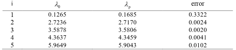
Table 1. Exact and approximate eigenvalues of the perturbed problem having five degrees of freedom. Here ₀ represents eigenvalues of the original problem, and _p eigenvalues of the perturbed problem.

i ₀ _p error

1 0.₁₂₆₅ ₀.₁₆₈₅ ₀.₃₃₂₂

2 2.₇₂₃₆ ₂.₇₁₇₀ ₀.₀₀₂₄

3 3.₅₈₇₈ ₃.₅₈₀₆ ₀.₀₀₂₀

4 4.₃₆₃₇ ₄.₃₄₅₉ ₀.₀₀₄₁

5 5.₉₆₄₉ ₅.₉₀₄₃ ₀.₀₁₀₂

To be specific we take m₀1 and k₀1. Using the eig command of the matlab software, we can obtain the eigenvalues of the original problem. The natural frequencies of vibrations of this original problem are the square-roots of the eigenvalues. We also compute our stiffness response (22) to the change of mass. The results of eigenvalues are listed in Table 1. The average of eigenvalues of the original problem is 03.3533 The average of eigenvalues of the perturbed problem is p 3.3433.

The average error of the eigenvalues is 0.07, that is, about 2.09%.

Remark 2: With this final example we notice that the norm of M0 is 0.3 and the norm of M0 is 5 .

Here we have that the perturbation of the mass is about 6% of the norm of the original problem. Using our proposed formula, in order that we maintain the frequency is about the same as the original frequency the norm of K₀ is 0.8697 with a note that the norm of K₀ is 20.3509 . Here we have that the response of the stiffness is about 4.3%. As desired, small change of mass is responded with small change of stiffness in order that the new frequency is about the same as the original frequency.

4. Conclusion

We have proposed a formula to compute a first order approximation of the stiffness difference if the involved mass in the structural dynamics is changed. The formula is limited to the structural mathematical model without friction. The formula is derived from the scalar spring-mass model with its degree of freedom is one. We have shown that an extension of its use for problems of higher degree of freedom has been successful. We project that the formula is applicable for large size problems, as long as the mass perturbation is not so excessive.

Acknowledgments

This work was financially supported by Sanata Dharma University. The support is gratefully acknowledged by both authors.

References

[1] Avitabile P 2003 Sound Vib. January 2003 14

[2] Kalaycioglu T and Ozguven H N 2014 Mech. Syst. Sig. Process. 46 289 [3] Mazlan A Z A and Ripin Z M 2016 JSCE 230 130

[4] Mottershead J E and Friswell M I 1993 J. Sound Vib. 167 347 [5] Ouyang H and Zhang J 2015 Mech. Syst. Sig. Process. 50-51 214

[6] Skafte A, Aenlle M L and Brincker R 2016 Smart Mater. Struct. 25 025020

[7] Supriyadi B 1993 Recalage des modeles de batiment (Ecole Centrale de Lyon: PhD Thesis) [8] Cha P D and Solberg K A 2008 Int. J. Mech. Eng. Educ. 36 160

[9] Chen J C and Wada B K 1977 AIAA J. 15 1095 [10] Nad M 2007 ACM 1 203

[11] Sestieri A 2000 Sadhana 25 247