8
and Production
C O N C E P T S
● Individual Proprietorship ● Partnership
● Corporation ● Unlimited Liability
● Limited Liability ● Factors of Production
● Inputs ● Primary Factors of Production
● Labour ● Capital
● Land ● Production Function
● Cobb-Douglas Production Function ● CES Production Function
● Total Product or Total Physical Product ● Marginal Product or Marginal Physical Product
● Average Product or Average ● Total, Marginal and Average Returns Physical Product
● Total Product Curve or Total Physical ● Marginal Product Curve or Marginal
Product Curve Physical Product Curve
● Average Product Curve or Average ● Law of Diminishing Marginal Product, Physical Product Curve Law of Diminishing Marginal Returns
or Law of Diminishing Returns
● Returns to Scale ● Increasing Returns to Scale
● Constant Returns to Scale ● Diminishing Returns to Scale
● Linearly Homogeneous Production Function ● Isoquant or Production Indifference Curve
● Economic Region of Production ● Technique (as opposed to Technology)
● Marginal Rate of Technical Substitution ● Leontief Technology
● Input Coefficient ● Input-Output Analysis
● Iso-cost Line ● Cost Minimisation Problem
● Normal Input ● Inferior Input
● Expansion Path
C
hapters 2, 4 and 5 dealt with demand for commodities by households. It is firms who supply goods and services to the market. While in Chapter 3 we learnt about the supply curve, in this chapter and the next few we will analyse the behaviour of firms with respect to how much they produce and supply to the market.However, before getting into various concepts and analyses, it will be useful to know what types of firms operate in an economy in terms of ownership, manage-ment and liability, and the general goal of a firm. Surely, the business of a road-side ice-cream vendor is different from that of firms like Mother Diary, Amul, Kwality, Vadilal, Baskin-Robins or Nirulas that produce ice-cream.
TYPES OF FIRMS
There are mainly three types of firms: individual proprietorship, partnership and corporation. Individual proprietorship refers to any single-owner or single family-owner business. Most small businesses are of this kind. If you own a small stationery shop, then you are an individual proprietor. Management typically lies with the owner or the entrepreneur. If anything goes wrong with the business in terms of defaulting on loans or negligence in paying taxes, the individual owner is entirely responsible or ‘liable.’ For a business to operate legally (whether it is an individual proprietorship or not), it has to be registered with the Registrar of Companies (ROC).1
Apartnershipis one in which a group of people run a business as partners. They are co-owners and mostly manage the firm directly. A partnership typically involves a small business. Many professional groups, for example, lawyers and chartered accountants, form partnerships. The key feature of a partnership firm is that each partner is totally liable, or has unlimited liability,as does the owner in an individual proprietorship. It means, for example, that if there is an outstanding payment that needs to be made and the other partners cannot pay for some reason, then you as a partner are entirely responsible.
In a corporation, there is typically a difference between ownership and man-agement. The shareholders are the owners and they appoint a board of directors, among whom some (like the CEO, Chief Executive Officer) are directly responsi-ble for the operations of the enterprise. Limited liabilityis a crucial feature of a corporation. It means that a shareholder is responsible/liable for payments only to the extent of his ownership share in the company. For example, if some out-standing payment has to be made, say Rs 50 lakh, and there is no other way to finance it other than collecting it from the owners, then if you own 10 per cent of shares in the company, your liability cannot exceed Rs 5 lakh. Among corpora-tions, there are private limited companies and public limited companies. In the
former, the shares are held among a few and any new shareholder has to be approved by the existing shareholders. Shares are not traded in the stock market. A private limited company can ‘go public’ and become a ‘public limited company’ by offering an IPO (initial public offering). The general public can buy its shares. All big private companies (for example, Reliance, Infosys) fall into this category. Some public sector firms like BHEL, MTNL and Indian Oil are also public limited companies. In public sector firms, the government holds a large percentage of shares and appoints its own people to manage the company. Unlike private limit-ed companies, public limitlimit-ed companies are supposlimit-ed to follow more norms and they are subject to more regulatory scrutiny.2
GOAL OF A FIRM
In consumer theory, the basic behavioural assumption is that consumers max-imise their surplus or utility. What is the objective of a firm? In economics, the prevailing assumption is that a firm’s goal is to maximise its profit. This is quite intuitive since the entrepreneur’s or the owner’s benefit lies in the profit income the firm generates.
However, for corporations in which ownership is separated from management, it is argued that the management may not be necessarily maximising the share-holders’ profits. Typically the shareholders are large in number and do not have adequate information about the true merits and demerits of important decision-making. Thus, the management can survive and do well for itself as long as it pro-vides some minimum acceptable returns to the shareholders, thereby ‘keeping them happy.’ Rather, the argument goes, managers make decisions so as to max-imise sales or revenues—to which their remuneration, perks and reputation are linked—subject to some minimum profit constraint.
However, the assumption one should make for analysing a firm’s behaviour must rest ultimately not on how intuitive or reasonable the objective of the firm appears to an individual or an expert, but whether the assumption leads to good predictions about the firm’s behaviour in terms of the observables. By this criterion, it turns out that the profit maximisation assumption is as good as any other alternative assumption that has been proposed in the literature on the the-ory of the firm.
Therefore, profit maximisation remains the dominant assumption regarding the goal of a firm and this will be assumed in this chapter and elsewhere in the book.
While the goal of profit making is certainly pertinent for a private firm, how about a public sector firm? The very adjective ‘public’ and its ownership (at least a
large fraction of it) by the government strongly suggest that such a firm is supposed to work in the ‘public interest’ and not necessarily to maximise profits. Whether such firms in India have truly worked in the public interest or not is debatable, but it is a fact that a majority of these were incurring heavy losses consistently over decades. It is an open secret that a significant proportion of employment in these sectors was politically rather than economically motivated. Surely, these firms were not operating on the principle of profit maximisation.
But as you know, many losing public sector enterprises in India have been disinvested (sold to private parties). Further, the remaining firms are now under increasing pressure to show results in terms of revenues raised and profits earned. Hence, of late, profit maximisation appears as a good working hypothesis for the functioning of public sector firms as well.
FACTORS OF PRODUCTION OR INPUTS
We now begin the analysis of production. Our starting point will be to understand technology—not in an engineering sense but in terms of the patterns of relation-ship between various inputs used in the production process and output.
Of course, different goods have different technologies of production. Wheat and computers are not produced by the same technology. Even the same good is not produced by a single technology. Rice or paddy is produced in many parts of India by relatively labour intensive methods whereas highly mechanised methods of agriculture are used in many developed countries.
Even though specific technologies may differ, there are, however, common qualitative elements across the production processes of various goods. For instance, whether it is kulfi, hair-cutting, bicycles or rockets, the amount produced within a given time period depends, among other things, on how many workers are employed and how many hours they work. Similarly, it may depend on machinery, equipment, building, land, raw materials and so on. Various things that go into a production process are called, in general, factors of productionor inputs.
Various equipment and machines are termed as capital. Landrefers to areas on the ground (as in agriculture as well as spaces like rooms, flats and buildings.3 Here and elsewhere we shall use the terms ‘factors’ and ’inputs’ interchangeably.
PRODUCTION FUNCTION
The technical process that links inputs to output of a good is called the production function of that good. It is defined as the technological relationship between inputs and output—giving the maximum output that can be produced from vari-ous input combinations.
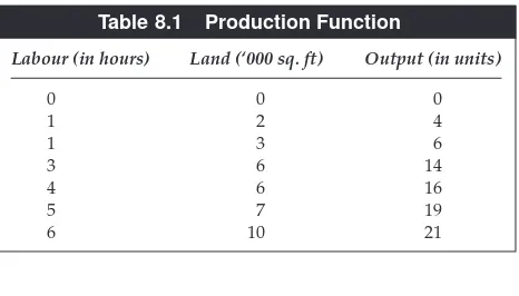
Suppose a firm employs two inputs, say, labour and land, measured respec-tively in hours and thousand square feet. Various input-to-output combinations are given in Table 8.1. Labour of 1 hour and 2,000 sq.ft of land produce, at the most, 4 units of output; 5 hours of labour and 7,000 sq.ft of land produce, at the most, 19 units of output; and so on. Table 8.1 describes a production function.
Note the following.
(a) It is normally assumed that inputs work to the best of their efficiency. Hence, instead of ‘maximum output’, we just say output.
(b) The notion of production function is not limited to two inputs. There can be many, including several types of capital or several different skills of labour. (c) Table 8.1 lists only some, not all, possible combinations of inputs and output. (d) In fact, very generally, one can write a production function as a
mathe-matical function. If we denote various inputs as x1, x2, x3,…, x
n,and the
output by y, then, algebraically, we can write the production function as y= f(x1, x2, …, x
n). Indeed, this is analogous to the utility function
intro-duced in Chapter 4. As an example, suppose that there are two inputs,
Table 8.1 Production Function
Labour (in hours) Land (‘000 sq. ft) Output (in units)
0 0 0
1 2 4
1 3 6
3 6 14
4 6 16
5 7 19
6 10 21
3Some economists include a fourth primary factor of production: entrepreneurship, referring to the owner(s) of a firm, who
1 and 2 and If A=10, x1=9 and x2=5, then we have output, The two often used production functions in applied eco-nomic analysis are the Cobb-Douglas and CES production functions.4For
two inputs, say L(labour) and K (capital), these technologies are given by,
RETURNS TO AN INPUT
A production function given in tabular form as in Table 8.1 or in algebraic form does not say much about how any single input contributes to production. This is measured by varying one input while keeping other inputs fixed. There are three important concepts here.
Total Physical Product, Marginal Physical Product
and Average Physical Product
The total product or total physical product of an input, denoted by TPP, is defined as the total output associated with a given level of employment of the input in question. The marginal productor the marginal physical product(MPP) is defined as the increase in the total physical product per unit increase in the employment of an input. In both these definitions, it is presumed that other input levels are unchanged. Let the input in question whose employment is varying be called a ‘variable input.’
Finally, the average productor the average physical product(APP) is defined as the TPPper unit of the variable input, that is, APP = TPP/L, where Lstands for the variable input.
The three notions just defined are also respectively called total,marginal and average returnsto an input. These notions are not unrelated to the production function; they do characterise it.
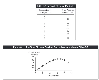
Table 8.2 shows a TPP schedule, where the variable input, L, is called labour. The graph of a TPP schedule gives the total physical product curve. Figure 8.1 shows the TPPcurve for the TPPschedule given in Table 8.2. Why the TPPcurve shapes this way will be discussed later.
The marginal physical product, MPP, can be obtained from the total physical product, TPP,just as marginal utility is derived from total utility. For example, the
Cobb-Douglas: CES:
y AL K A
y A
= > > >
=
α β α β
, 0, 0, 0
[[δLθ+(1−δ)Kθ ν θ]/ ,A>0 0, <δ θ, <1,ν>0.
y=10 9 5( + )=80.
y=A x( 1 +x2).
4Recall that in Chapter 4 we talked about the Cobb-Douglas utility function. In fact, the Cobb-Douglas utility function is an
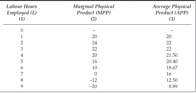
MPPat L =2, which is 24, is equal to the difference between TPPat L =2, which is 44, and TPPat L =1, which is 20. The MPPschedule corresponding to Table 8.2 is given in column (2) of Table 8.3. The APPschedule is given in column (3) of Table 8.3; for each value of L, it is equal to TPPdivided by Lin Table 8.2.
We see that both MPP and APP initially increase and then decrease. Further, after a certain point, MPPbecomes negative. The graphs of an MPPschedule and an APPschedule are respectively called the marginal physical product curveand the average physical product curve. These graphs based on Table 8.3 are shown in Figure 8.2. Both are inverse U-shaped curves since MPP and APP initially increase and then decrease.
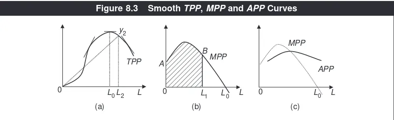
If the variable input can be measured continuously like decimal points on the real line—rather than discrete numbers like 1, 2, 3, …and so on—the TPP, MPP and APPcurves will look smooth. Figure 8.3 depicts such curves.5
0 25 50 75 100 125
0 2 4 6 8 10
Labour Hours Total Physical
Product
Figure 8.1 The Total Physical Product Curve Corresponding to Table 8.2
5Ignore for now the tangents drawn on panel (a), the shaded area in panel (b) or the superimposition of the MPP curve in panel (c).
Table 8.2 A Total Physical Product Labour Hours Total Physical Employed (L) Product (TPP)
0 0
1 20
2 44
3 66
4 86
5 102
6 112
7 112
8 100
Note that the concepts of TPP, MPPand APPapply to all inputs, not just labour.
But the important point is that they measure how output changes with respect to any particular input, ‘one at a time,’ when the other input levels are fixed.
Interrelationships
(i) Although both MPPand APPare derived from TPPby definition, there are
a few interrelationships. Given any one of these three, the other two can be derived. Suppose MPPs are known to us. Since these are additions to TPP,
we can get TPP by adding MPPs, that is, TPP is the sum of MPPs. In
Table 8.3, at L = 3, the MPPs add up to 20 + 24 + 22 = 66. Check from
Table 8.2 that at L=3, TPP=66. If the MPPcurve is smooth, then the sum
of MPPs is nothing but the area under the MPPcurve and it equals TTP.
Table 8.3 Marginal Physical and Average Physical Schedules Labour Hours Marginal Physical Average Physical Employed (L) Product (MPP) Product (APP)
(1) (2) (3)
For instance, as shown in Figure 8.3(b), the TPP of employing L1units of labour is equal to the area 0ABL1. Once we get TPP, we can readily obtain
APPby applying its definition.
Similarly, if the APPs are known, we get TPPby multiplying APPwith the
level of employment. Then MPPs are obtained by applying its definition.
(ii) APPis equal to the slope of the ray from the origin to the point on the TPP
curve. For instance, in Figure 8.3(a), at L = L2, TPP = y2. Thus APP =
L2y2/0L2, which is simply the slope of the ray 0y2from the origin.
(iii) By definition, MPPis the addition to the TPPas the variable input increases
by one unit. Hence, if the TPP curve is smooth, MPPis the derivative of
TPP, equal to the slope of the TPPcurve, as shown in Figure 8.3(a). It then
follows that TPPincreases, remains constant or decreases as MPPis
posi-tive, zero or negative.
(iv) Note in Figure 8.3(c) that the MPPcurve cuts the APPcurve at the maximum point, that is, as APPrises (to the left of the maximum point), MPP>APP
and as APPfalls (to the right of the maximum point), MPP < APP. The
reason behind this is mathematical not economic and the mathematical logic is spelt out below through an example.
Suppose you are a very enthusiastic college teacher, very eager to know how your students did in a challenging test you gave last week. After checking each script you enter its score (marks) into the computer and the computer gives you the average score of all scripts you have checked so far. You have already checked 9 scripts and the average is 85 (out of 100).
Suppose that the next (10th script) receives 91. Without entering this number in the computer, can you say if the new average will be higher or lower than 85, the old average? Yes, you can—the average will be higher. So far the average was 85 and thus if the last (‘marginal’) student’s score is greater than the old average, it
will push up the average. This means that (i) if the ‘average’ is increasing, the
‘marginal’ must be greater than the average.
If instead, the 10th student had scored anything less than 85, by the same logic,
it would have pulled down the average. This implies that (ii) if the ‘average’ is
decreasing, the ‘marginal’ must be below the average.
MPP
Now you join statements (i) and (ii), substitute ‘average’ for APPand ‘marginal’ for MPP. It follows that if APPis rising, MPP> APP, and if APPis falling, MPP< APP. This, in turn, implies that the MPPcurve must cut the APPcurve at the lat-ter’s maximum point.
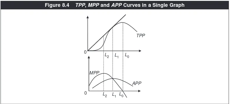
Various relationships among TPP, MPPand APPare summarised, so to speak, in Figure 8.4. The top part graphs the TPPcurve and the bottom part the correspon-ding MPPand the APPcurves. Between the levels of employment from 0 to L
2, TPP
is increasing at an increasing rate (that is, the slope is rising). Accordingly, in the bottom panel MPPis increasing. From L
2to L1, TPPincreases at a decreasing rate
(that is, the slope decreases) and accordingly, in the bottom panel the MPP falls. At L=L
0, the slope of the TPP curve, equal to the MPP, is zero. Beyond L0, TPP
slopes downwards and thus MPP<0. The APPbeing equal to the slope of the ray from the origin to the point on the TPP curve, we see in the top part that it increases between 0 to L
1and falls thereafter. We also see that at L =L1, APPis
maximum and equal to the slope of the TPPcurve (MPP); in other words, MPP= APP, where APPachieves its maximum.
LAW OF DIMINISHING RETURNS
Now we discuss the economic reason behind why various curves are shaped the way they are. As it turns out, the pattern that MPPinitially increases, then dimin-ishes and finally becomes negative is the key. This pattern has a name: the law of diminishing marginal productor the law of diminishing marginal returnsor, briefly, the law of diminishing returns. According to this law, keeping the employ-ment of other inputs fixed, as more of a particular input is used in production, after a certain level, its marginal physical product decreases. The logic behind this law is the following. When the employment of a single input gradually increases while all other inputs are kept unchanged, the factor proportions among other inputs and
L0 L1
APP
L2 L1
0
L2
0 L
0
MPP
TPP
the input in question become initially more suitable for production because the scarcity of the (needed) variable input gradually falls. This tends to increase the marginal product. But, after a certain level, the variable factor can work with other given inputs only less efficiently (as other inputs become relatively scarce), that is, factor proportions become increasingly unsuitable for production. This implies that the marginal product of a factor would fall as more of it is used.
The MPPinitially increasing and then falling implies an inverse U-shaped MPP
curve, that is, the law of diminishing returns explains this shape of the MPPcurve. In turn, this explains the particular shape of the TPPcurve and the inverse U-shape of the APPcurve.
Two points need to be noted with respect to the law of diminishing returns. First, diminishing returns to a factor may set in right from the beginning, that is, MPPmay be diminishing throughout. In that case, the point L2in Figure 8.4 essentially coincides with the origin.
Second, a profit-maximising firm will never hire so much of any input such that its MPPis negative. Why? Because, if it does, it always can employ a bit less of the input in question, which would increase output and revenue from sales as well as save costs (as less of the input is employed and paid) and thus increase profits. A firm will continue to do this until the MPPis no more negative. However, see Clip 8.1 for statistical evidence on the existence of negative marginal product in a public sector enterprise.
Clip 8.1 Evidence on Negative Marginal Product
It is an open secret that there is or used to be excess employment in public sec-tor enterprises run by the government. The reason behind this is not hard to seek—some jobs are/were handed out on the basis of political rather than profit considerations. Can such excess employment be so high that the mar-ginal product of a certain kind of labour employed is negative? It is very easy to conjecture on this but very difficult to back it up with ‘hard’ evidence.
However, an econometric study by Das and Sengupta (2004) finds evidence on negative marginal product of certain type of workers in the government steel sector in steel plants under SAIL (Steel Authority of India Limited). On the basis of data on employment and productivity in 16 blast furnaces over the period 1991–97, the authors have found the evidence of negative marginal product for non-executive workers. The output elasticity of such workers was −0.17, that is,
10 per cent increase in such workers would decrease output by 1.7 per cent. The good news, however, is that, lately, the government steel sector has become profitable and casual empiricism tells that it has become more efficient.
Reference:
Mathematically Speaking
Returns to an Input and the Relationship
between APP and MPP
As we have seen earlier, we can write a general production function as y=f(x
1, x2, ..., xn), where yis the output and x1, x2, ..., xnare the employment levels of inputs 1, 2, 3, ..., n. Let the inputs 2, 3, ..., nbe fixed, while x1may vary. That is, let the employment of only input 1 vary. Then the functional relationship between x1and
yis the TPPof input 1, which we can write as y= f(x1), where the ‘dot’ means that the other inputs are fixed. APPis defined as y/x1= f(x1)/x1. We can write this sim-ply as f/x1. Similarly, MPPis the partial derivative of ywith respect to x1, that is,
∂f/∂x
1. Positive MPPmeans ∂f/∂x1>0. Diminishing marginal product means that the second derivative is negative, that is, ∂2
f/∂x
12<0. Differentiate the APPwith respect to x1. We have,
This proves that if APPis increasing (or decreasing), that is, dAPP/dx1is posi-tive (or negaposi-tive), MPP> (or <) APP.
* * * * * *
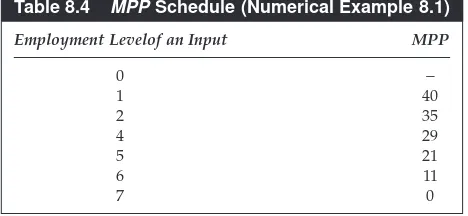
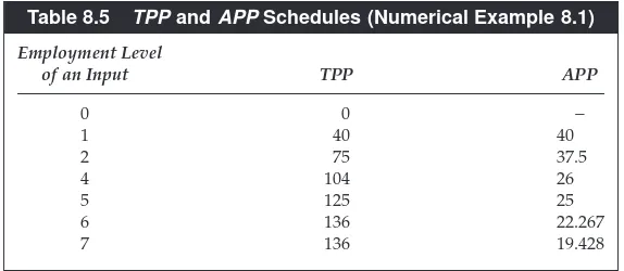
NUMERICAL EXAMPLE 8.1
The MPPschedule of a variable input is given in Table 8.4. Assuming that the TPP
at zero level of the input is zero, derive the TPPand the APPschedules.
Since TPPis the sum of MPPs, TPPat the employment level equal to 1 is equal to TPP at zero level of employment (which is 0) plus the MPP of input at the employment level 1 (which is 40); that is, it is equal to 0 + 40 = 40. Likewise, the
TPPat the employment level of 2 units is equal to 40 + MPPat this level of employ-ment (which is 35) = 75. TPPs at higher levels of employment are calculated
dAPP
Table 8.4 MPP Schedule (Numerical Example 8.1)
sequentially and listed in the middle column of Table 8.5. Once we know the TPPs, APPs can be obtained by dividing TPPs by the respective levels of employment.
These are listed along the last column of Table 8.5. (At zero level of employment,
APPis not defined.)
RETURNS TO SCALE
We have studied the concepts that capture the contribution of any single input towards production. This does not mean at all that a firm can vary only one input at a time. When market conditions or technologies change, a firm would very well adjust many inputs. For instance, if a garment factory finds a cheaper source of getting cotton, it would like to expand its production by hiring more workers (labour) and buying more sewing machines (capital) as well. There are concepts that capture the joint contribution of inputs towards output.
Assume that a firm is not employing any input so much that its marginal prod-uct is negative (a profit-maximising firm would not do it anyway). Suppose that it increases the employment of all inputs by a given proportion (for example, by 10 per cent). The output will surely increase because the marginal product of each input is positive. But by how much? If it increases more than proportionately (for example, by more than 10 per cent), we say that there are increasing returns to scale. If the output rises but less than proportionately, there are decreasing returns to scale. Finally, if it increases exactly proportionately, there are constant returns to scale. Formally, we say that there are increasing returns to scale, constant returns to scale or decreasing/diminishing returns to scalewhen,as all inputs increase proportionately, the output increases more than, exactly or less than proportion-ately respectively.
Note the following:
(a) The words ‘diminishing’ and ‘decreasing’ used above do not mean that
output decreases when all inputs increase.
(b) These concepts relate again to the production function. A production
func-tion may exhibit one type of returns to scale at all input levels or may exhibit any combination.
Table 8.5 TPP and APP Schedules (Numerical Example 8.1)
Employment Level
of an Input TPP APP
0 0 −
1 40 40
2 75 37.5
4 104 26
5 125 25
6 136 22.267
(c) In particular, if a production function satisfies constant returns to scale throughout, it is also called a linearly homogeneous production function. For example, suppose there are two inputs, labour (L) and capital (K), and the production function is Cobb-Douglas, given by y=L0.6K0.4. Starting with any initial values of Land K, check that if Land Kare doubled, yis also doubled.
2, ..., λxn). Increasing, constant or decreasing returns to scale are differentiated
on the basis of whether f(λx
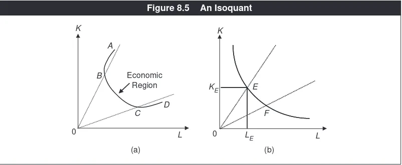
If there are two inputs, the production function can be shown graphically by an isoquant, defined as the locus of combinations of inputs, which give rise to the same level of output. If, for example, the two inputs are labour and capital, vari-ous combinations of Land Kthat produce, say, 60 units of output define the iso-quant for output = 60. In principle, it is like an indifference curve. That is why an isoquant is also called a production indifference curve.
How does an isoquant look like? Suppose the MPPs of both inputs are positive. Then, starting from a given combination of inputs producing a given amount of output, if the employment of one input is increased, there is more output. Thus, if the output has to be brought down to its original level, the amount used of the other input has to be reduced. In other words, an increase in one input must be matched with an appropriate decrease in the other so that the output is unchanged. This implies that the isoquant will have a negative slope. If we consider a very high level of employment of an input such that its MPPis negative, then an increase in one input must be associated with an increase in the other such that the output remains the same. Accordingly, the isoquant will have a positive slope. Overall then, an isoquant will look like the line ABCDdrawn in Figure 8.5(a). However, as discussed earlier, a profit-maximising firm will never use an input such that its
MPP is negative. Thus the segments AB and CD on the isoquant ABCD are not
operational for such a firm. The segment BC is the only economic region of production. For this reason, from now on, an isoquant will be assumed to be a downward sloping curve, as shown in Figure 8.5(b).
A whole isoquant reflects technology whereas a technique refers to the pro-portion of inputs used at a givenpoint on the isoquant. Referring to Figure 8.5(b), at point E, for example, 0LEamount of labour and 0KEamount of capital are used. The capital/labour ratio is 0KE/0LE. Since 0KE=ELE, this ratio is equal to ELE/0LE, which is the slope of the ray from the origin 0E. Similarly at point F, the capital/labour ratio is the slope of the ray 0F. Clearly, the ratio is higher at pointE
than at point F(as 0Eis steeper than 0F). We say that, compared to F, Einvolves a relatively more capital-intensive or a relatively less labour-intensive technique.
Once you see the similarity between an isoquant and an indifference curve, you realise that the economic analysis of production has some similarity with that of consumer behaviour. A collection of isoquants in a single graph is called an isoquant map. An isoquant to the right of a given isoquant represents a higher output. Two isoquants cannot intersect. Remember the definition of marginal rate of substitution of one good for another. The equivalent concept here is the mar-ginal rate of technical substitution(MRTS), referring to the rate of substitution between inputs so that the output is unchanged. For instance, the MRTSof input 1 for input 2 equals the amount of input 2 that needs to be foregone per unit increase in input 1 so that the output remains unchanged. MRTSis equal to the ratio of marginal products just as the MRSin consumer theory is equal to the ratio of mar-ginal utilities. If, for example, there are two inputs, labour and capital, then the
MRTSof labour for capital is equal to the MPP of labour divided by the MPPof capital.
Remember the assumption of diminishing MRS in consumer theory, which implied that an indifference curve is convex to the origin. Here we assume dimin-ishing MRTSand it implies that an isoquant is convex to the origin, as shown in Figure 8.5(b).
0 L
K
0 B
C D
L K
A
Economic Region
(b) (a)
KE E
F
LE
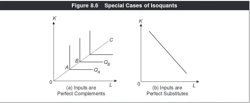
Also remember the special cases of indifference curves along which the goods were perfect complements or perfect substitutes. Similar looking isoquants reflect inputs being perfect complements and perfect substitutes of each other. These are shown in panel (a) and panel (b) respectively in Figure 8.6. Indeed, they are analo-gous to Figure 4.7 in Chapter 4. Perfect complementarity means that the inputs are used in a fixed proportion with each other. This implies that if the employment of one input is increased and yet output is to be kept unchanged, no amount of any other input can be sacrificed. Thus, MRTS=0. In Figure 8.6(a) this proportion is
indicated by the ray 0C. Any deviation from this proportion leads to no increase
in output. This explains the vertical and flat portions of the isoquants. Such a tech-nology is called the Leontief techtech-nology, named after Wasily Leontief, a Nobel laureate in economics, who extensively used the assumption of this technology in his research. Perfect complementarity also means that the ratio of an input to output, called the input coefficient, is constant. The study of Leontief technology is also sometimes called an input-output analysis. On the other hand, when an isoquant is a straight line, as shown in panel (b), its slope is fixed. Thus MRTSis
positive and constant. Since, irrespective of how much of each input is being used initially, a given amount of one input needs to be sacrificed per unit increase in the other input so as to keep the output unchanged, the inputs are perfect substitutes of each other.
However, from now on, we assume diminishing MRTSand accordingly assume
downward sloping, convex isoquants as in Figure 8.5(b).
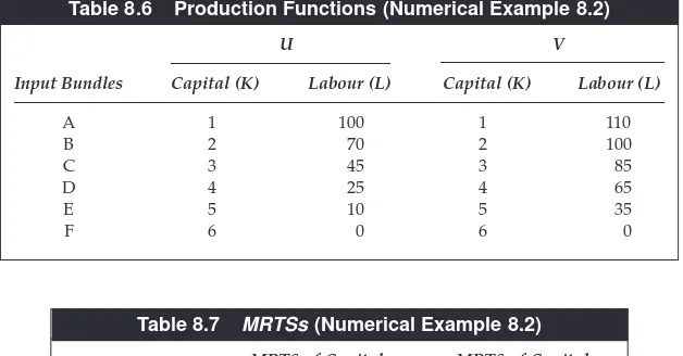
NUMERICAL EXAMPLE 8.2
In Table 8.6, the input bundles in the columns Uand Vdefine isoquants for two
dif-ferent levels of output. Derive the marginal rates of technical substitution of capi-tal for labour along both isoquants. Is the assumption of diminishing marginal rate of technical substitution satisfied?
0
(b) Inputs are Perfect Substitutes A
B
0
C
QB
(a) Inputs are Perfect Complements
QA
K
L K
L
MRTSmeasures the rate of sacrifice of an input when the employment level of
another input increases. The MRTSof capital for labour is the amount of labour
sacrificed per unit increase in capital as we go down the input bundles in Table 8.6. Along isoquant U, from input bundle A to B, it is equal to 100 – 70 = 30 units of
labour. From the input bundle B to C, it is 70 – 45 = 25 units of labour, and so on. Table 8.7 lists the MRTSs. We observe that MRTSis decreasing along the isoquantU
but not decreasing along the isoquant V. (In the analysis of this chapter we
disre-gard isoquants of the type V.)
ISO-COST LINE
We now characterise costs through what is called an iso-cost line (although there are a lot more concepts on costs to be introduced in the next chapter). Suppose labour and capital are the two inputs. Labour costs Rs wper hour and renting
cap-ital (for example, a truck) costs Rs rper unit. Thus, wand rare the respective
fac-tor or input prices for labour and capital. We define an iso-cost lineas the locus
of combinations of inputs whose total costs are the same.
In our example, the total cost = wL (cost of labour) + rK (cost of capital).
Consider the iso-cost line for total cost equal to, say, Rs 1,000. Let w= 50 and r= 40.
Various combinations of Land Ksuch that wL+ rK= 1,000 define the iso-cost line
for total cost = Rs 1,000.
Table 8.7 MRTSs (Numerical Example 8.2)
MRTS of Capital MRTS of Capital for Labour along for Labour along Input Bundles Isoquant U Isoquant V
A to B 30 10
B to C 25 15
C to D 20 20
D to E 15 25
E to F 10 30
Table 8.6 Production Functions (Numerical Example 8.2)
U V
Input Bundles Capital (K) Labour (L) Capital (K) Labour (L)
A 1 100 1 110
B 2 70 2 100
C 3 45 3 85
D 4 25 4 65
E 5 10 5 35
Clearly, along an iso-cost line, if the firm hires more of one input, it must hire less of the other. Indeed you can see that the iso-cost line is identical to the price line studied in consumer theory, except that total cost substitutes income, factor prices substitute product prices and we are talking about demand for inputs rather than demand for goods. Thus, like the price line, the iso-cost line is a downward sloping straight line. Figure 8.7 shows an arbitrary iso-cost line. Just as a slope of the price line equals the ratio of product prices, the slope of the iso-cost line is equal to the ratio of factor prices. In Figure 8.7 where labour is measured along the x-axis and capital along the y-axis, it is equal to the wage/rental ratio, that is, w/r.
While an iso-cost line is defined on the basis of a given total cost, the total cost itself may change, depending on how much a producer is willing to spend on inputs. In other words, iso-cost lines can shift just as the price line in consumer theory does. Different levels of total cost imply different iso-cost lines.
Consider an increase in the total cost. This will lead to a parallel rightward shift of the iso-cost line. Similarly, a decrease in total cost will lead to a parallel leftward shift of the iso-cost line. A change in a factor price can also shift an iso-cost line. Suppose there is an increase in the wage rate, w.If the firm hires labour only, with the same amount of total cost, it can hire less of it (as labour is more expensive). This will shift the intercept of the iso-cost line on the axis measuring labour towards the origin. In Figure 8.7 the iso-cost line will become steeper.6
COST MINIMISATION
By using the various concepts and assumptions at our disposal, we now analyse a decision-making problem facing a firm. Suppose a firm has committed itself to pro-duce a given amount of output.7Which combination of inputs should it choose?
L 0
w r K
Figure 8.7 An Iso-cost Line
6Similarly, an increase in r will shift the intercept of the iso-cost line on the axis measuring capital and in Figure 8.7 the
iso-cost line will become flatter.
Turn to Figure 8.8(a). Suppose the output to be produced is y0. The firm can choose any point on the isoquant representing y0. Suppose it selects the input com-bination at point A. The total cost of this is indicated by the iso-cost line passing through this point, namely aa. Consider another combination B. Its total cost is shown by bb. Since the line bblies to the left of the line aa, the combination Bcosts less than the combination A. Similar calculation can be made from any other com-bination on the isoquant.
As stated earlier, the firm’s objective is to maximise profits. Profits, by definition, are equal to total sales revenues minus the total cost of inputs. Obviously, the higher the costs, the less are the profits. Hence, maximising profits implies that the firm must choose that input bundle which costs the least among those that can produce the output. We now go back to Figure 8.8(a) and ask which input bundle entails the minimum total costs, given that the firm is producing y0. The answer is the tangency point C. Because at any other combination of inputs (such as Aor B), the iso-cost line will be at a higher level compared to that at C. The input levels, LC of labour and KCof capital associated with the tangency point C(Figure 8.8(b))then constitute the cost-minimising choice of inputs.
In general, we say that the optimal or the cost-minimising choice of inputs is governed by the condition that the iso-cost line be tangential to the isoquant. Since the slope of the former is the input price ratio and that of the latter is the MRTS (equal to the ratio of MPPs), we can write the condition elaborately as,
Cost-minimisation Condition:
MRTS=ratio of MPPs =factor price ratio. (8.1)
When, for example, the factors are denoted by Land K, with wand ras the respec-tive factor prices, we can write this condition as:
A Change in an Input Price
Having derived the cost-minimising condition, we can analyse how a change in a factor price or the output level can affect the optimal choice of inputs.
Suppose labour becomes cheaper.8This will make iso-cost line flatter (as its slope
equals w/r). Turning to Figure 8.9, suppose Cis the original point of choice and ccis the associated iso-cost line. With a lower value of w, the new iso-cost lines will be flatter than ccsuch as, ee, or any other line parallel to ee. The new cost-minimising input bundle is the tangency point between the isoquant y0and the iso-cost line ff,
which is parallel to ee. This is the bundle D. Compared to C, the new input combi-nation has more labour and less capital. This makes sense because labour being relatively cheaper now, the firm is hiring more labour and less capital—that is, it is employing a more labour-intensive technique.
A Change in Output
Suppose the firm decides to produce a higher quantity, y1, than the original out-put y0 (while input prices are unchanged). This means a higher isoquant. The effects are shown in Figure 8.10. In both panels, the point Cis the original cost-minimising input bundle. In panel (a), the new bundle is indicated at A. Compared to the original input bundle, the firm hires more of both inputs. Panel (b) illustrates the case where the firm employs more of one input and less of the other. You can notice that the effect of an increase in output is similar to that of an income effect in demand theory. Like normal and inferior goods, we define normal and inferior inputs. An input is said to be normal or inferior as, at constant factor
prices, the demand for it increases or decreases with output. In panel (a), both
8It could happen if, for example, workers from outside migrate into the area. L 0
D K
e
C c
e
f c f
y0
inputs are normal whereas in panel (b), labour is the normal input while capital is the inferior one.
Note, however, that irrespective of whether some inputs are inferior, a higher output is always associated with a higher iso-cost line, that is, total cost always increases with output.
Suppose we extend this exercise and let output increase continuously. The effects are shown in Figure 8.11. The cost-minimising points are C
1, C2, C3and so on. If we join these points, the line (0E) is called the expansion path, defined generally as the locus of cost-minimising input bundles at different levels of out-put, given the input prices. The expansion path indicates a firm’s pattern of hiring inputs as it plans to expand its production.
L 0
E
C2 K
C3
C1
Figure 8.11 Expansion Path
(b) One Input Inferior (a) Both Inputs Normal
0
B C
L K
y0
y1
0 K
L C
A
y1
y0
Mathematically Speaking
Isoquants, Iso-cost Lines and Cost Minimisation
With two inputs 1 and 2, we can write the production function as y= f(x1, x2). Totally differentiating this we have dy= (∂f/∂x1)dx1+(∂f/∂x2)dx2. Along an isoquant, there is no change in output, that is, dy= 0. Hence (∂f/∂x1)dx1+(∂f/∂x2)dx2= 0. We can rewrite this as:
(8.3)
This proves that an isoquant is downward sloping and its slope = MRTS, which is, in absolute value, equal to the ratio of marginal products.
Let w1and w2denote the respective input prices. The total cost has the expres-sion C=w1x2+w2x2. Totally differentiating it, dC=w1dx1+w2dx2. On an iso-cost line dC= 0 since Cis constant. Hence, w1dx1+w2dx2= 0, implying
This proves that the iso-cost line is downward sloping and the absolute value of its slope is equal to the factor price ratio.
Cost minimisation states that C=w1x1+w2x2is minimised along an isoquant. Keeping in view (8.3),
If Cis minimised, dC/dx1=0. This implies that the term inside the brackets [] is zero, that is,
The last equation is same as the cost-minimisation condition stated in (8.2).
* * * * * *
NUMERICAL EXAMPLE 8.3
Consider the input bundles along the isoquant U in Table 8.8. Suppose the price of capital services is r=Rs 60 and that of labour services (the wage rate) is w=Rs 5. Which of the input bundles among A to F minimises the total cost of producing the
Economic Facts and Insights
● Most businesses are individual proprietorships.
● In individual-proprietorship and partnership firms, each owner has
unlim-ited liability, meaning that if the company is due for a payment and other owners are not in a position to pay (for example, someone dies or is currently
Table 8.8 Cost Minimisation along the Isoquant U
Total Cost: Total Cost: Input Bundles K, L r ==60; w ==5 r ==80; w ==5
A 1, 100 560 580
B 2, 70 470 510
C 3, 45 405 465
D 4, 25 365 425
E 5, 10 350 450
F 6, 0 360 480
output associated with isoquant U? Suppose capital becomes more expensive—
rincreases from Rs 60 to Rs 80. Now, which input bundle minimises the total cost? Compare the new cost-minimising input bundle to the old cost-minimising input bundle.
This is straightforward. For each bundle, we know the level of each input and its price. Multiplying them gives the total cost of hiring that input. Summing it over the two inputs gives the total cost of the input bundle. For instance, consider input bundle B having 2 units of capital and 70 units of labour. With r= 60, 2 units of cap-ital will cost 120 and with w= 5, 70 units of labour will cost 350. Thus the total cost of input bundle B is equal to 120 +350 =470. Table 8.8 enumerates the total cost of all
input bundles at the two input-price combinations. When r= 60 and w= 5, the total cost is the minimum at the input bundle E; the minimised total cost is equal to 350. When r = 80 and w = 5, the total cost is minimised at the input bundle D; the minimised total cost is equal to 425.
Compared to the input bundle E, the input bundle D has less capital and more labour because hiring capital is costlier. Put differently, capital is relatively more expensive and labour is relatively cheaper and hence the firm hires less capital and more labour. Furthermore, in the new situation, in absolute terms, one input price is the same while the other is higher. This is why the minimised cost in the new situation (425) is greater than that in the original situation (350).
E
E X
X E
E R
R C
C II S
S E
E S
S
8.1 What are the differences between a partnership form of business and an individual proprietorship?
8.2 What is the difference between a partnership business and a corporation? 8.3 ‘A private firm makes its decisions with the objective of maximising its
prof-its.’ Comment.
8.4 ‘In the real world, many firms go out of business. Thus, profit maximisation is a bad assumption.’ Defend or refute.
residing in a foreign country), then a owner who is available is responsible for the entire amount due.
● Limited liability and separation of management from ownership are the
salient features of a corporation.
● In predicting the behaviour of a firm, profit maximisation has worked as
good as other alternative assumptions as the goal of a firm.
● In India, public sector firms are becoming more and more profit-oriented. ● Primary factors provide their services to a production activity whereas raw
materials are totally used up in a production process.
● The contribution of an individual input to output is captured by the notions
of total physical product, marginal physical product and the average phys-ical product.
● The marginal physical product and the average physical product curves are
inverse U-shaped curves because of the law of diminishing returns.
● The basis of the law of diminishing returns lies in that as more and more of
a single factor is used in production, the proportion of this factor with respect to other factors becomes higher and, therefore, less suitable for pro-duction.
● A profit-maximising firm will not use any input to the level that its marginal
product is negative.
● A profit-maximising firm will employ input combinations that minimise
total cost at any given level of output.
● The cost-minimisation condition is one where the marginal rate of technical
substitution, which is same as the ratio of marginal products of inputs, is equal to the ratio of input prices.
● Given an output, an increase in an input price would lead a firm to use less
of that input. Thus an increase in the wage rate will lead a firm to use a less labour-intensive (that is, a more capital-intensive) technique. Similarly an increase in the rent will induce a firm to use a less capital-intensive, that is, a more labour-intensive technique.
● An increase in output may or may not lead to an increase in the