SCHOOL OF ECONOMICS DISCUSSION PAPER 98/10
TAXATION, FISCAL ILLUSION AND THE DEMAND FOR
GOVERNMENT EXPENDITURES IN THE UK: A TIME-SERIES
ANALYSIS
by
Abstract
Public choice analysts have often argued that the level of government spending will reflect voter-taxpayer’s demand for public goods, while the fiscal illusion literature has argued that certain features of the tax structure affect voter’s perceptions of their tax burden causing them to underestimate how much they are paying for public goods. In such cases public expenditure is typically predicted to be greater than that proposed by simple ‘decisive-voter’ demand models. In this paper we test whether standard fiscal illusion arguments, typically examined in a cross-section context, for local public goods, can help to explain the time-series behaviour of national-level public expenditure in the UK over the period 1955-94. The sources of fiscal illusion which we examine are: the visibility of taxes; the extend of deficit finance; revenue complexity; and tax elasticity. If public expenditure is determined by a fully-informed, rational decisive voter then it should be independent of these ‘tax structure’ variables. We find fairly robust evidence, however, that increased use of less visible (indirect) taxes and deficit financing was associated with increased use of less visible (indirect) taxes and deficit financing was associated with increased levels of spending. Closer examination suggests that deficit financing is more a short-term necessity in the fact of shocks than an illusory plan by government. However, it seems that in the UK case, governments relying more on indirect taxes than direct taxes have, other things equal, been able to sustain higher government expenditures.
Acknowledgements
1. INTRODUCTION
It has long been alleged that the public sector tends to grow faster than the economy as a whole. More than a century ago, Wagner asserted that this tendency was inevitable. With the increasing availability of time series data, many writers have tested Wagner’s Law, narrowly defined as asserting that the income elasticity of demand for government output is greater than unity, but there appears to be little empirical support for this strict definition (Diamond, 1989; Gemmell, 1990, 1993). Alternative explanations for public sector growth contend that this tendency is not inevitable. Peacock and Wiseman (1961), for example, argued that external shocks, such as wars, caused sudden increases in public spending which did not revert back to its pre-shock level once the shock had passed. During ‘non-shock’ periods there was no necessary tendency for the public sector share of national income to increase; rather it tended to hover around its existing share.
Public choice theorists have argued that the level of government spending should reflect voter-taxpayer’s demand for public goods. In this vein, models of the demand for public expenditure were developed by Borcherding and Deacon (1972) and Bergstrom and Goodman (1973). However since as early as Puviani (1903), various analysts have suggested that certain features of the tax structure affect voters’ perceptions of their tax burdens so that they may underestimate how much they pay for publicly-provided goods. Such fiscal illusion arguments often lead to the prediction that observed expenditure will be greater than that derived from a simple 'decisive voter' model. In this paper we adopt a public choice approach to try to explain trends in UK government expenditure (as a measure of the size of the public sector) by adapting fiscal illusion models of local government to a national context. To explore these arguments we add a number of fiscal illusion variables to a model of the demand for public goods in order to try and explain the time-series behaviour of public expenditure in the UK over the period of 1955-94.
2. FISCAL ILLUSION AND PUBLIC SPENDING
Fiscal illusion is typically alleged to arise if certain features of the tax structure lead taxpayers to underestimate how much tax they truly pay, creating ‘excess’ demand for government-provided goods, ie. more public expenditure is demanded than would be in the absence of fiscal illusion (for detailed reviews see Oates, 1991a; Dollery and Worthington, 1996). Frequently proposed sources of fiscal illusion are: the degree of visibility of taxes; the extent of deficit finance; revenue complexity; and tax elasticity. The essence of these arguments is as follows. The greater the share of ‘less visible’ taxes in tax revenue (Pommerehne and Schneider, 1978), and of deficit finance relative to spending (Goetz, 1977), the greater the likelihood that taxpayers underestimate the tax-price and vote for higher levels of government expenditure. A more complex tax system will make it more difficult for voter-taxpayers to identify their true tax burden hence increases the likelihood of underestimating the tax-price of government-provided goods (Wagner, 1976). The more elastic the tax system the more responsive is revenue to growth in national income, hence it is easier to sustain a higher volume of public spending if income is growing (Buchanan, 1967).
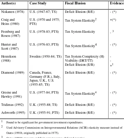
Table 1: Time-Series (and Pooled Time-Series) Studies of Government Expenditures and Fiscal Illusion
Author(s) Case Study Fiscal Illusion Evidence
Niskanen (1978) U.S. (1947-67; TS) Deficit Illusion (R/E) - (*)
Craig and
U.S. (1978-83; PTS) Tax System Elasticity - 3
Hunter and Scott (1987)
U.S. (1976-83; PTS) Tax System Elasticity4 - (*)
Henrekson (1988)
Sweden (1950-84; TS) Tax System Complexity (H) Visibility (DRT/TT)
U.S. (1977-84; PTS) Tax System Elasticity4 - (*)
Tridimas (1992) U.K. (1955-88; TS) Deficit Illusion (R/E) - (*)
Ashworth (1995) U.K. (1955-91; PTS) Deficit Illusion (R/E) - (*)
1 Found to be significant for government investment expenditures.
2 Used Advisory Commission on Intergovernmental Relations (ACIR) elasticity measure instead of Oates (1991b, originally published in 1975).
3 Oates (1991b) measure and their own measures all found negative.
4 Used tax cuts as dependent variable which is affected positively by tax progressivity.
Key:
TS: Time-series; PTS: Pooled Time-series.
R: Government Revenues, E: Government Expenditures, H: Herfindahl Index, DRT: Direct Taxes, TT: Total Tax Revenues.
The evidence for deficit illusion appears contrary to the Ricardian Equivalence Theorem, which holds that individual consumers recognise the government’s intertemporal budget constraint and are thus aware that any change in current taxes must be offset by a change in future taxes. If this holds, we would expect government expenditures to be negatively related to deficits, as voter-taxpayers will be reluctant to incur future tax liabilities. Buchanan and Wagner (1977) however argued that voters tend to discount future tax liabilities, so budget deficits can support excess government spending because they reduce the perceived price of public services to the current generation of voters. The evidence in Table 1 supports this more myopic view.
The inclusion of tax elasticity as a determinant of public expenditure derives from the seminal study of Oates (1991b) who found a positive and significant effect of a measure of tax elasticity on general government expenditures. Subsequent empirical evidence has been mixed: Craig and Heins (1980) found support for Oates; Misiolek and Elder (1988) found a positive and significant relation between tax elasticity and tax revenues, but the effect on government expenditures was not significant. Baker (1983), Feenberg and Rosen (1987), and Heyndels and Smolders (1994) did not find significant results for elasticity; DiLorenzo (1982), Greene and Hawley (1991) and Hunter and Scott (1987) all found a negative but significant relationship between elasticity and government expenditures.
The pioneering study of the effect of revenue complexity on government expenditure is Wagner (1976) who found a negative relationship between the simplicity of the revenue structure and total expenditures. The Herfindahl index, suggested by Wagner, has subsequently been used by others as a measure of revenue system complexity: Baker (1983), Breeden and Hunter (1985), and Heyndels and Smolders (1994), for example, found a positive and significant effect of revenue complexity, while Misiolek and Elder (1988) and Henrekson (1988) found no support for the hypothesis.
It is clear therefore, even from this brief review, that the empirical evidence for the influence of fiscal illusion on public expenditure, however measured, is ambiguous. In the UK context, previous time-series analyses have considered only deficit illusion but generally found support for the hypothesis. Below we consider whether there is robust evidence for more extensive fiscal illusion effects on UK public expenditure trends. First we introduce the key relevant features of the UK tax structure.
Trends in Tax Structure in the UK
Figure 1 shows that government expenditure tended to rise steadily from 1955 until the early 1980s, after which the ‘Thatcher era’ witnessed a marked reduction in the expenditure/GDP ratio, though this was largely reversed in the 1990s. Revenue tended to keep pace with spending until the late 1960s (running ahead in 1968-71); a deficit emerged in the light of the oil crisis which peaked in 1974, was reduced significantly in the early 1980s, re-emerged, was eliminated in 1987-88 and re-emerged again. Three broad patterns can be identified from Figure 1: (i) revenue and expenditure tracked fairly closely over 1955-72; (ii) although a deficit wedge was inserted, revenue and expenditure still tended to track over 1973-1989; and (iii) since 1990 the two have diverged, with revenue falling while spending rose, implying a steadily increasing deficit.
The elements of fiscal illusion identified earlier may offer insights into these trends in at least two ways. First, governments can avail of fiscal illusion to increase spending, either by allowing the deficit to increase or by an appropriate tax structure, such as more reliance on less visible taxes. Second, faced with a sudden need to increase spending (eg. a Peacock-Wiseman effect), governments may have recourse to fiscal illusion to disguise from voters the need to finance the increase. Thus, an increased deficit is an obvious response to an external shock which immediately increases the demand for spending (while it is difficult to adjust tax revenue quickly, and may be politically difficult to cut spending). The fiscal illusion hypothesis would suggest in this context that, over time, to maintain spending and reduce the deficit (because of its macroeconomic effects), the tax structure will evolve in an ‘expenditure-supporting’ manner.
over 1955-72 and 1978-94. Direct taxes on personal income (PIT), the relatively visible taxes in the UK context (as the amount paid is printed on pay slips and tax returns), showed more movement: rising steadily from about 20 per cent of revenue in 1955 to 25 per cent in 1961 and 30 per cent by 1973, and remaining within a band of about 25-30 per cent over 1977-94. During the crisis of 1974-78, both these taxes moved ‘out of their bands’ but that period can be considered an aberration.
The other major revenue sources exhibit gentle trends. Social Security Contributions (SSC), the relative visibility of which is questionable, rose from a share of about ten to over 15 per cent. Corporate income taxes (CIT), which are not paid directly by voters and therefore should be considered invisible to individuals, moved around mostly within a 5-10 per cent band. Non-tax revenues (NTR), which are also in principle 'invisible' (from the fiscal illusion perspective) declined slightly in importance from about twelve to eight per cent of total revenue. An examination of Figure 2, however, does not reveal any simple influence of fiscal illusion, in the sense that it is not clear that the share of less visible taxes rose as expenditure increased, though our empirical analysis can address the question with greater rigour.
The observation of remarkable stability in the tax structure is consistent with the literature on party political influences on British taxes. Rose (1984) argued that the impact of parties on trends in the economy is minimal compared with secular forces, and that similarly, contrary to their rhetoric, parties have no partisan influences on trends in the level and composition of taxation. Karran (1985) found no evidence for a significant impact of parties on taxation. Although, at least prior to Blair, Labour was perceived to be a higher tax party than the Conservatives, the evidence generally suggests that taxes tended to rise, and their composition remained stable, irrespective of which party was in power. Morrissey and Steinmo (1987) argue that the impact of parties is rather on the distribution of the burden within taxes: Conservative governments tended to levy lower tax rates on the rich, increased nominal rates of consumption tax, and encouraged corporations to distribute their profits to shareholders. Labour governments were more likely to increase income tax rates on the rich and consumption tax rates on luxury goods, and encouraged corporations to reinvest.
effects of fiscal illusion. However, the more general implication of the partisan influence literature is that the party in power does not affect general trends in revenue or its composition, and we do not anticipate partisan influences in our empirical work.1
3. A MODEL OF EXPENDITURE AND FISCAL ILLUSION
The demand for government-provided goods can be modelled following Borcherding and Deacon (1973) and Bergstrom and Goodman (1973) as:
Gi = a Yiα Pgiβ, i=1,2,...,N (1)
where Gi is voter-taxpayer i’s consumption of government provided goods, Yi is i’s income, Pgi is i’s tax-price paid for Gi. The coefficients α and β capture income and price elasticities of demand for government-provided goods, respectively.
The tax-price is specified as Pgi =Ti C Nη, where Ti is i’s tax share, C is the unit cost of G, and N is population with the degree of publicness η. Borcherding and Deacon (1972) assume non-discrimination in taxation specifying the tax-price, Pgi =C Nη-1 as all pay the same amount of tax.2 Eliminating Pgi from the model gives equation (2):
Gi = a Yiα Cβ Nβ(η-1) (2)
In a time-series context, if there is a productivity lag in the public sector, the implied difference between private and public sector prices should be taken into account: government expenditures must be appropriately deflated as the variables in the model are defined in real terms, and a measure of public-private price differences should be included in (2). Using relative prices and aggregating to express demand in terms of total expenditures:
G = a Yα Prβ Nφ where φ = (β+1)(η-1)+η-α (3)
where G and Y are total government expenditures and gross domestic product, respectively, both in real terms, and Pr (=C/Px) is the relative price where Px is price
1 Nevertheless we test for this later, and confirm that party dummies are not significant.
2 If the same amount of tax is paid by every voter-taxpayer, then the tax share is computed by the following formula: Ti=(T/N)/T= N
-1
of private sector goods.3 Specification (3) is the standard model of demand for government-provided goods used in most previous empirical studies based on the median voter model.
Such a specification adopts the theory of democratic process in which it is assumed that citizens are fully aware of the costs and benefits of government-provided goods. However, as noted above, several studies within the public choice field have challenged this assumption, suggesting that voter-taxpayers may not be aware of their ‘true’ tax-prices because of some features of the tax structure. The relevant arguments in the case of central government expenditures are deficit illusion (D), the invisibility of indirect taxes (V), the complexity of the tax system (H), and the tax elasticity (L). D is typically proxied by the ratio of government revenues to government expenditures, V by the ratio of ‘less visible’ taxes to government revenues,
H by a Herfindahl concentration index, and L by the ratio of income taxes to government revenues.
To incorporate this formally into our analysis let the perceived tax price be a function of the perception parameter (Π) and the ‘true’ tax-price, as P ˆ gi = Π Pgi, where Π is a function of D, V, H, and L as follows:
Π = Dπ1 Vπ2 Hπ3 Lπ4 (4)
Replacing Pgi by P ˆ gi in (1), and substituting (4), the model (3) can be written in the following logarithmic form:
lnG = lna + α lnY +β lnPr + φlnN
+δ1 lnD + δ2 lnV + δ3 lnH + δ4 lnL + u (5)
where δ1, δ2, δ3, and δ4 represent π1β, π2β, π3β, and π4β respectively. The coefficients δ1 and δ3 are predicted to be negative while δ2 and δ4 are predicted to be positive. This is the model we estimate below.
3 It should be noted that total nominal government expenditure, E, is given by G
i Pgi N
η
, where Gi
4. DATA AND ILLUSION MEASURES
Data for UK general government expenditure and revenue for the period of 1955-94 are used in our analysis. Government expenditure (G) in real terms is the sum of three categories: government final consumption at 1990 prices, about half of total government outlays; government gross domestic fixed capital formation, deflated by the GDFCF deflator; and transfers (consisting of current grants and subsidies, capital transfers and debt interest), deflated by the consumer price index. Gross domestic product (Y) is also at 1990 prices, while the relative price (Pr) is approximated by the ratio of the public sector deflator (computed as the weighted average of the three government expenditure deflators mentioned above ) to the GDP deflator.
As identified in equation (4), four measures are used to capture fiscal illusion. Deficit illusion (D) is captured by the ratio of revenue to expenditure: a value greater than unity implies a budget surplus, and the lower the value below unity the greater the deficit, thus the anticipated coefficient is negative. The value for D is plotted in Figure 3. In line with our discussion of Figure 1, one can identify four distinct periods: 1955-1968, when the deficit tended to move around zero (i.e. D = R/E moves around unity); 1968-73, a period of turmoil; 1974-89, when the deficit was steadily reduced; and post-1989, when the deficit has increased dramatically. Of course, it should be acknowledged (and we will return to this in discussing our results) that movements in the deficit may well reflect the unforeseen impact of macroeconomic shocks rather than any government intention to use the deficit as part of an illusory plan to increase spending beyond the level that would be supported by fully informed voters.
To measure tax system elasticity we follow Oates (1991b) and use the ratio of personal income taxes to total government revenues (L). It should be noted however that L will reflect more than simply the ‘automatic effects’ (elasticity) of the tax system. Firstly, discretionary changes in tax rates, thresholds etc. will also affect L; indeed Gemmell (1997) estimates that the elasticity of income taxes has fallen since the 1960s so that the revenue share of total income taxes may be an increasingly poor proxy for tax system elasticity. Secondly, to the extent that income taxes are relatively elastic, fiscal illusion arguments suggest that an increased income tax share will be associated, ceteris paribus, with increased expenditures. However, to the extent that income taxes are relatively visible, fiscal illusion arguments suggest an increased share will reduce expenditures. Thirdly, in the UK tax system, where personal income and expenditure taxes are the dominant revenue sources, changes in the expenditure tax share, tend to mirror changes in income taxes (see Figure 2). Indeed, since the two are highly negatively correlated (r = -0.86) we must be cautious about using both fiscal illusion variables in our regressions (see below).4
The complexity of the tax system (H) is measured by the Herfindahl concentration index: the sum of squares of the shares of various tax categories. Twelve categories of government revenues are available to compute H: (i) income tax on the personal sector, (ii) income tax on companies, (iii) income tax on non-residents, (iv) social security contributions, (v) expenditure tax on durable goods, (vi) expenditure tax on tobacco, (vii) expenditure tax on alcoholic drinks, (viii) expenditure tax on petrol and oil, (ix) expenditure tax on food, clothing, fuel and power, (x) expenditure tax on services (vehicle excise duty and other services), (xi) other expenditure taxes (on capital formation, companies and public corporation, and overseas sector), (xii) other government revenues. In fact, we experiment with two alternative computations of H: (i) using all twelve taxes, and (ii) aggregating the various expenditure taxes into a single expenditure tax category and calculating H from the resulting five taxes.
In a time-series context, where the number of revenue categories does not change much in the period of this study, H essentially reflects the relative magnitudes of major revenue categories, and consequently is highly correlated with both V and L. When the twelve categories mentioned above are used, H reflects the trends in L (the ratio of personal income tax) and r(H, L) = 0.99. On the other hand, when the various expenditure taxes are aggregated, H primarily reflects the trends in V (the ratio of
expenditure taxes) and r(H, V) = 0.65. Thus, in a time-series context with a fixed number of taxes as in the UK, the complexity of the tax system (as measured by a Herfindahl index) cannot readily be separately identified from invisibility/elasticity aspects. We are therefore unable to explore the effects of tax complexity in our regressions analysis below. The sign predictions for our variables in equation (5) are:
income (Y) positive; population (N) positive; relative price (Pr) negative; deficit (D) negative; invisible taxes (V) positive.
The coefficient on income taxes (L) is expected to be positive if 'elasticity' effects dominate, but is predicted to be negative if the measure primarily reflects the visibility of direct taxes.
5. EMPIRICAL RESULTS
Prior to Tridimas (1992) and Ashworth (1995) most time-series studies used OLS techniques to analyse government expenditures. However, as these techniques assume the data generating process to be stationary (which it is not), it is now known that standard diagnostic tests may fail, and the results may not be interpreted confidently. An ad hoc partial adjustment mechanism and a first order autoregressive structure is used by Tridimas (1992) to analyse data from the UK for the period 1955-88. Although previous empirical specifications are rejected by Tridimas’ findings, it is argued by Ashworth (1995) that the ad hoc dynamic specifications may still be misleading. Instead, Ashworth uses cointegration techniques, and extends the period of analysis to 1991. However, the only fiscal illusion variable included in either study is the deficit illusion measure, D. We follow a similar approach to Ashworth in this paper, extending the period under investigation further, to 1994, and exploring a range of fiscal illusion variables.
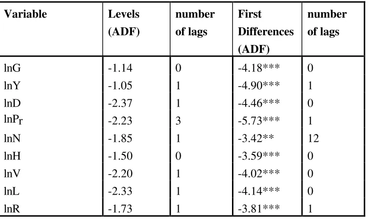
The variables in the model developed in Section 3 are first tested for stationarity both in levels and first differences, as seen in Table 2, where all the variables were found to be I(1).5 The next step is to test these variables for cointegration; we use the Johansen procedure applied to equation (5), omitting lnH for the reasons discussed earlier. In specifying invisible taxes, V, we noted earlier that expenditure tax (ET),
Table 2: Stationarity Tests
** (***) = Significant at 5(1)%. Critical values are -2.93 and -3.58 at 5% and 1% respectively. All tests were also run including a time trend; however none of the variables was found to be trend stationary.
Table 3: Cointegration Tests Using the Johansen Approach
Rank=r λλmax λλmax
(T-nm)
CV(5%) λλtrace λλtrace (T-nm)
CV(5%)
Variables in the Model: lnG, lnY, lnPr, lnN, lnD, lnV, lnL
r=0 73.28 60.12 45.3 166.5 136.6 124.2 r<=1 39.80 32.66 39.4 93.25 76.51 94.2 r<=2 24.36 19.99 33.5 53.45 43.85 68.5 Variables in the Model: lnE, lnY, lnPr, lnN, lnD, lnL
r=0 62.57 52.95 39.4 123.6 104.6 94.2 r<=1 32.28 27.31 33.5 60.99 51.61 68.5 r<=2 17.04 14.42 27.1 28.71 24.30 47.2 Variables in the Model: lnG, lnY, lnPr, lnN, lnD, lnV
r=0 71.42 60.43 39.4 139.4 118.0 94.2 r<=1 34.96 29.58 33.5 67.98 57.52 68.5 r<=2 18.73 15.85 27.1 33.02 27.94 47.2 Variables in the Model: lnE, lnY, lnPr, lnN, lnD, ln(ET/R), ln(SSC/R), ln(NTR/R).
r=0 74.26 59.03 51.4 202.4 160.9 156.0 r<=1 44.02 34.99 45.3 128.2 101.9 124.2 r<=2 36.69 29.17 39.4 84.13 66.88 94.2
corporate income tax (CIT), and non-tax revenues (NTR) may each be considered relatively invisible, and can create illusion. In the UK, SSCs could also be considered in this category. Further tests show that the CIT/Revenue ratio is stationary [ie. I(0)] so that it cannot cointegrate with I(1) variables.6 We therefore initially include three revenue categories (expenditure tax, non-tax revenues, and SSCs) in our definition of
V, examining sensitivity to the definition later.
Notwithstanding the fairly high negative correlation between lnV and lnL noted earlier, we begin by including both variables in our search for a cointegrating vector, and also excluding each in turn. The trace and maximum eigenvalue statistics, using maximum likelihood estimation, are reported in Table 3. The null hypothesis of “no cointegration” is rejected in all cases, suggesting that there exists at least one cointegrating vector.
On the question of whether lnV and/or lnL should be included in the cointegrating vector, when both are included coefficient estimates of 2.35 and 0.36 are obtained respectively suggesting, plausibly, that there are strong 'invisibility' effects from expenditure taxes. Ceteris paribus on this, the small positive coefficient on lnL could be interpreted as capturing residual 'elasticity' effects. When lnV is omitted from the cointegrating vector the parameter on lnL becomes -0.47, suggesting that 'visibility' effects from direct taxes dominates any 'elasticity' effects. When only lnL is included in cointegrating regressions however, other parameters are often wrongly signed (population becomes negative or relative prices become positive), and the inclusion of
∆lnL in the associated ECM is not supported. This is not the case for lnV. To test more formally for the inclusion of lnV and lnL in the cointegrating relationship, we conducted the Likelihood Ratio tests suggested by Johansen and Juselius (1992), testing the null hypotheses: δi = 0 (i = 2, 4) in equation (5). These strongly supported the inclusion of lnV in the regression but the exclusion of lnL7.
Following the arguments of Ashworth (1995) and Maddala (1992) that both the cointegrating vector and the ECM should inform the choice of the preferred model, we therefore prefer the vector excluding lnL. Further analysis supports the null
6 The ADF statistics for ln(CIT/R) and ln(SSC/R) are -3.14 and -2.18 respectively.
hypothesis of a “unique cointegrating vector” from both trace and maximum eigenvalue statistics.8 The preferred cointegrating regression is:
lnG = 0.81 lnY - 0.58 lnPr+ 1.65 lnN - 0.44 lnD + 1.67 lnV (6)
The positive signs on the coefficients for income and population, are in line with the previous findings of Diamond (1989), Tridimas (1992), and Ashworth (1995), though direct comparison can be made only with Ashworth (1995) who uses a similar method. The income coefficient here is somewhat lower than obtained by Ashworth (who obtains values of 0.89 and 0.97 in alternative specifications) though, like Ashworth (1995), a likelihood ratio test suggests that we cannot reject the null hypothesis that the coefficient on income equals unity. Nevertheless, since government expenditures appear to increase proportionately (or less than proportionately) with national income the simple Wagner's Law hypothesis is clearly rejected.9
Regarding the degree of publicness, η, this must be extracted from φ in equation (5) using the expression [(β+1)(η-1)+η -α] from equation (3). This yields η = 2.03 which is outside the expected range between zero and unity. Nevertheless, similarly large values have been found in previous studies (see Gemmell, 1990; Ashworth, 1995) and the results here tend to support the evidence of previous studies that, overall, government-provided goods are highly ‘private’ in nature.10
The effect of relative prices is found to be negative and price-inelastic demand for government-provided goods is supported. The negative sign confirms both Diamond and Ashworth’s findings, while Tridimas found a positive sign. It is well known that the relative price of government-provided goods demonstrates a secular upward trend over time in the UK (as in many other countries), whether due to ‘real’ or purely statistical reasons. The evidence here would appear to suggest that, ceteris paribus,
8 There is some weak evidence from the maximal eigenvalue test that there are two cointegrating vectors in the VAR model. However, this is rejected by other diagnostics; the null hypothesis of a ‘unique cointegrating vector’ is accepted by the LR-test(=0.28; CV[10, 5%]=18.3). Furthermore, Reimers (1992) suggests that in case of small samples, the Johansen procedure over-rejects when the null is true. Thus, the number of parameters to be estimated in the model are also taken into account, and an adjustment is made for degrees of freedom by replacing T by T-nm, where n is the number of variables in the model and m is the number of lags in the model. A unique cointegrating vector is accepted by the modified statistics (see Table 3).
9 The restriction imposed on the β matrix is rejected at 1% level (LR-Test=35.1, CV(10, 5%)=18.3).
10 Since η is determined by a combination of the coefficients on P
rand N, both of which show some
this has had a reductive effect on public expenditure presumably because resistance from voters against rising (nominal) public expenditures forces governments to respond with compensating reductions in real government output, in order to minimise these expenditure increases.
The negative effect of the tax ratio, lnD, is also in line with previous findings, and appears to support the public choice argument for deficit illusion: over the long-run there is a higher demand for government expenditures when a lower proportion is financed by taxes. This is consistent with the argument that voter-taxpayers do not fully perceive their future tax liabilities, posing a challenge to Ricardian Equivalence. However, prior to examining the short-run dynamics, such an interpretation may be premature and this will be discussed further below.
The proxy for (in)visibility, lnV, has the predicted positive sign, being consistent with the fiscal illusion hypothesis that voter-taxpayers demand more government expenditure when tax structure shifts towards a higher share of indirect taxes (plus other less visible taxes). Investigating the relative roles of the components of lnV
suggests that it is expenditure taxes which have the strongest revenue effects. The cointegrating vector with the three separate revenue components is (diagnostics are reported in Table 3):
lnG = 0.72 lnY - 0.59 lnPr + 1.70 lnN - 0.44 lnD + 0.98 ln(ET/R) + 0.43 ln(SSC/R) + 0.23 ln(NTR/R) (7)
The long-run impact on expenditures of switching tax structure towards expenditure taxes (and implicitly away from direct taxes) appears to be more than twice the effect of increasing social security contributions and roughly four times the effect of increasing non-tax revenues. That is, in public choice terminology, expenditure taxes are particularly ‘invisible’ and appear to be able to support ‘excess’ expenditure.
Notice also that this is not merely an association of a rising indirect tax share over time with rising expenditures; despite the introduction of VAT in mid-1970s, the share of indirect taxes has not been increasing over our period of investigation (the introduction of VAT appeared to halt a prior long-term decline in the expenditure tax share).
Though it can be argued that switches to invisible (ie. indirect) taxes have permitted increased expenditures (compared to what they otherwise would have been), this should not be interpreted as indicating substantial scope for additional government spending by further moves towards indirect taxation. Clearly the marginal
expenditure impact of raising V above its current share of around 43 per cent could be substantially less and could be expected to fall further as V approaches its limit of unity
The next step is to estimate the error correction model (ECM) to test for short-run adjustment towards long-run equilibrium, and to explore the nature of fiscal illusion (if any) in the short run. The results from the most parsimonious specification are as follows (t-statistics are in the parentheses):11
∆lnGt = -4.2 + 0.18∆lnYt-1 - 0.59∆lnPr,t-1 - 5.93∆lnNt - 0.41∆lnDt+
(-6.2) (1.49) (-2.44) (-3.82) (-5.24)
0.45∆lnVt-1- 0.27Ut-2 (8)
(3.52) (-6.23) R2=0.72, FAR=0.1(prob=0.91), χ
2
NORM=4.84(prob=0.09), FHET=0.82(prob=0.63)
The error correction term is negative and significant at one per cent level, and the magnitude of the corresponding coefficient shows that almost 30 per cent of any disequilibrium in the long run relationship between the variables is corrected within two years. The contemporaneous value of the tax ratio, lnD, is also significant, consistent with the findings of previous time-series models. The first lag of ∆lnV is also found to be significant, suggesting an illusionary effect from the indirect tax share in the short-run as well as the long-run.12
11 Various combinations of variables in contemporaneous and lagged values have been tried. The most parsimonious specification is reported here. All the diagnostics pass at 5% level of significance.
12 When the three revenue categories are included separately, the ratio of expenditure tax only is found to be significant in the short-run. The ECM results are as follows:
∆lnG = -2.85 + 0.17 ∆lnYt-1 -3.9 ∆lnNt -0.47∆lnDt +0.19 ∆ln(ET/R)t-1 -0.21Ut-2 (5.37) (1.29) (2.62) (5.8) (2.61) (5.39) R2=0.67, FAR=0.45(prob=0.64), χ
2
We would not be equally confident to interpret the significant contemporaneous value of lnD as support for fiscal illusion in the short-run, as the lagged values of lnD did not appear significant in any of the estimates, implying that any effect of deficits is realised in the same year. This could be explained by the determination of expenditures and revenues simultaneously, and is consistent with the observation that a shock leads to an increase in the deficit as revenue cannot quickly be increased, while expenditure is not easily reduced quickly. Of course, as noted earlier, higher levels of expenditures, if not matched by revenue adjustments in the current period, imply a lower tax ratio (D = R/G) which may appear as an inverse (contemporaneous) relationship between expenditures and the tax ratio (due to a direct 'accounting' effect, as distinct from an 'economic' or 'fiscal illusion' effect, on the budget deficit).
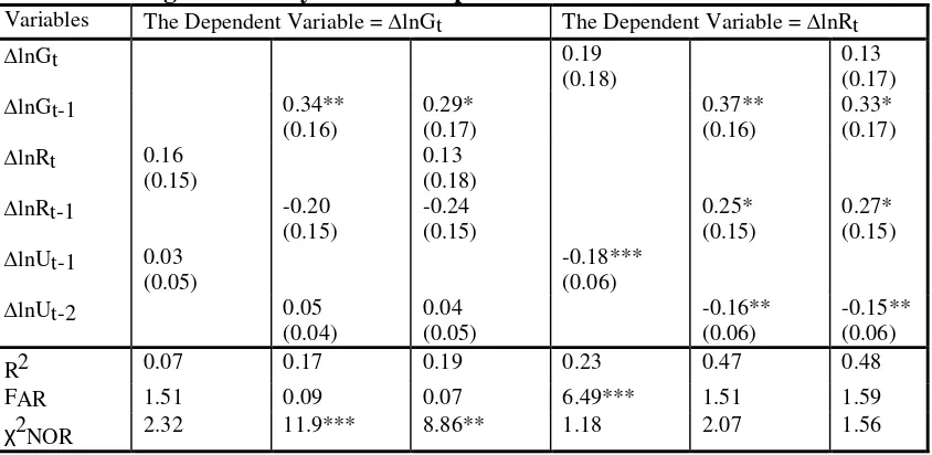
To explore the issue of the interaction between budget deficits and government expenditures further, we conduct Granger-causality tests on the two variables. As seen in Table 4, these support the conclusion that the direction of Granger causality is from expenditures (lnG) to deficits (lnD) rather than vice versa. When expenditures are taken as the dependent variable, lagged lnD is not significant; when the dependent variable is lnD, lnG is significant both in contemporaneous and lagged values. The evidence that lnGt is negatively associated with the tax/expenditure ratio is consistent
with the suggestion above that when governments increase expenditures, revenues do not rise commensurately in the same year. A similar conclusion was reached by Ashworth (1995: 13): ‘This would seem to be in line with the original Wagner view which recognises that there is not a smooth continuous rise in public activities but that revenue constraints limit public expansion.’ The positive effect of the first lag of expenditures on lnD is also consistent with the government budget constraint: governments cannot borrow forever, and revenues rise, or expenditure is adjusted to reduce the deficit, in later periods, though slowly.13
So, the mechanism behind the negative relationship between G and D (=R/G) is probably that the government increases expenditures (G); this consequently increases the deficit, ie. reduces the tax/expenditure ratio (D¬), and hence results appear as negative effect of D on G. The results from the causality tests are consistent with our explanation for the apparent significance of deficit illusion: governments do
utilise budget deficits, and this may imply a lower political risk, but usually in response to a shock which increases expenditure (or suddenly reduces revenue).
In testing for fiscal illusion using equation (5) in a time-series context, we have required that adjustments in tax or deficit variables precede adjustments to government expenditures, as a necessary condition for those to be regarded as capturing fiscal illusion effects. It could be argued of course that governments which are aware that it is easier to increase expenditures when the financing can be 'hidden' in deficits or
Table 4: Granger Causality Between Expenditures and Deficits
Variables The Dependent Variable = ∆lnGt The Dependent Variable = ∆lnDt
∆lnGt -0.81*** FAR 3.62** 0.09 0.30 6.49*** 0.61 1.59 χ2
NOR 6.79** 11.9*** 5.64* 1.18 0.32 1.56
Table 5: Granger Causality Between Expenditures and Revenues
Variables The Dependent Variable = ∆lnGt The Dependent Variable = ∆lnRt
∆lnGt 0.19 FAR 1.51 0.09 0.07 6.49*** 1.51 1.59 χ2
indirect taxes, are not bound by such temporal precedence. Thus governments may increase expenditures today, knowing that a combination of increased deficits and/or increased use of indirect taxes in the future can finance this. That is, if voters are relatively unaware of increases in deficits and indirect taxes they are also likely to be unable to associate these with expenditure increases in particular years. While this argument would allow us to interpret the deficit-expenditure interactions as consistent with the fiscal illusion hypothesis, it is also the case that the evidence is consistent with governments using deficits in a standard 'consumption smoothing' manner analogous to a private individual with no money illusion but volatile income levels. Since the present approach cannot discriminate between these alternative hypotheses, we are reluctant to interpret our results (on deficits) as evidence of fiscal illusion.
Finally, we noted earlier that some commentators have argued that the political party in government may influence expenditure levels. We have investigated this by adding (the first difference of) a dummy variable for periods of Labour government to the error correction representation of equation (8). Consistent with the arguments and evidence of Morrissey and Steinmo (1987), we find no support for the view that,
ceteris paribus, expenditure levels differ between party political regimes; in particular, they are not higher under Labour.14
6. CONCLUSIONS
This paper approached an explanation of trends in British government expenditure utilising public choice theories that the level of government spending should reflect voter-taxpayer’s demand for public goods. Such theories argue that certain features of the tax structure affect voter’s perceptions of their tax burden so that they underestimate how much they are paying for public goods. Such fiscal illusion implies that actual expenditure will be greater than predicted by a simple voter demand model. Previous public choice based studies of the demand for public expenditure have found mixed evidence for the impact of fiscal illusion, though none use the range of specifications of illusion variables employed here.
To test these theories we added fiscal illusion variables to a model of the demand for public goods using UK data for the period of 1955-94. The included sources of fiscal illusion were: the visibility of taxes; the extent of deficit finance; revenue complexity; and tax elasticity. The greater the share of ‘less visible’ taxes in tax revenue, and of deficit finance relative to spending, the greater the likelihood that taxpayers
underestimate the tax-price and vote for higher levels of government expenditure. A more complex tax system will make it more difficult for voter-taxpayers to identify their true tax burden and hence increases the likelihood of underestimating the tax-price of government-provided goods. The more elastic the tax system the more responsive is revenue to growth in national income, hence it is easier to sustain a higher volume of public spending (if income is growing) without generating adverse public reaction.
The results obtained are consistent with comparable studies of public expenditure. Our innovation was in a more complete specification of sources of fiscal illusion. We found quite consistent evidence that invisible taxes and deficit financing were associated with increased levels of spending, but for various reasons the measures of elasticity and complexity performed less well (largely because they were highly correlated with the measure of visibility). Closer examination suggested that the appropriate interpretation of deficit financing is less that it represents an illusory plan to hide expenditure increases from voters and more a short-term necessity when shocks cause (trends in) spending and revenue to diverge. The support for illusion due to invisible taxes is stronger. We found some evidence that governments relying more on indirect taxes than direct taxes have, other things equal, been able to sustain higher government expenditures. This is consistent with the fiscal illusion hypothesis that where public officials prefer a higher level of government spending they can focus on less visible taxes in order to obtain more revenues with less public reaction. We would not, however, argue that this necessarily offers a means to increase future expenditure beyond the levels currently supported by voter-taxpayers. The current indirect tax share is at the upper end of the historical range of observed values and it remains unclear whether still higher rates of indirect tax would allow these taxes to remain relatively 'invisible'. Our evidence would suggest however, that future governments pursuing a policy of switching the mix of taxes away from indirect taxes may find it more difficult (over the long-run) to sustain political support for a given aggregate
REFERENCES
Ashworth, J (1995). The Empirical Relationship Between Budgetary Deficits and Government Expenditure Growth: An Examination Using Cointegration. Public Finance, vol.50, no.1, pp.1-18.
Baker, S. H. (1983). The Determinants of Median Voter Tax Liability: An Empirical Test of the Fiscal Illusion Hypothesis. Public Finance Quarterly, vol.11, pp.95-108.
Bergstrom, T. C. and R. P. Goodman (1973). Private Demands for Public Goods. The American Economic Review, vol.63, pp.280-296.
Borcherding, T. E. and R. T. Deacon (1972). The Demand for the Services of Non-Federal Governments. The American Economic Review, vol.62, pp.891-901. Breeden, C. H. and W. J. Hunter (1985). Tax Revenue and Tax Structure. Public
Finance Quarterly, vol.13, pp.216-24.
Buchanan, J. M. (1967). Public Finance in Democratic Process, The University of North Carolina Press, Chapel Hill.
Buchanan, J. and R. Wagner (1977). Democracy in Deficit, Academic Press, New York.
Clotfelter, C. T. (1976). Public Spending for Higher Education: An Empirical Test of Two Hypotheses. Public Finance, vol.31, pp.177-95.
Craig, E. D. and A. J. Heins (1980). The Effect of Tax Elasticity on Government Spending. Public Choice, vol.35, pp.267-75.
Diamond, J. (1989). A Note on the Public Choice Approach to the Growth in Government Expenditure. Public Finance Quarterly, vol.17, pp.445-61.
DiLorenzo, T. J. (1982). Tax Elasticity and the Growth of Local Public Expenditure.
Public Finance Quarterly, vol.10, pp.385-92.
Dollery, B. E. and A. C. Worthington (1996). The Empirical Analysis of Fiscal Illusion. Journal of Economic Surveys, vol.10, no.3, pp.261-97.
Feenberg, D. R. and H. S. Rosen (1987). Tax Structure and Public Sector Growth.
Journal of Public Economics, vol.32, pp.185-201.
Gemmell, N (1990). Wagner's Law, Relative Prices and the Size of the Public Sector.
The Manchester School of Economic and Social Studies, vol.58, pp.361-77. Gemmell, N. (1993). Wagner’s Law and Musgrave’s Hypotheses. in N. Gemmell
(ed.), The Growth of the Public Sector, Edward Elgar, Aldershot.
Gemmell, N. (1997). Financing Future Public Expenditure: Will Tax Rates Have to Rise? A Research Report for BBC ‘Newsnight’.
Granger, C. W. J. and P. Newbold (1974). Spurious Regressions in Econometrics.
Journal of Econometrics, vol.12, pp.231-54.
Greene, K. V. and B. K. Hawley (1991). Personal Income Taxes, Elasticities and Fiscal Illusion. Public Choice, vol.72, pp.101-09.
Goetz, C. J. (1977). Fiscal Illusion in State and Local Finance. in T. E. Borcherding (ed.), Budget and Bureaucrats: The sources of Government Growth. Duke University Press, Durham, pp.176-87.
Hall, S. G. (1991). The Effect of Varying Length VAR Models on the Maximum Likelihood Estimates of Cointegrating Vectors. Scottish Journal of Political Economy, vol.38, no.4, pp.317-23.
Harris, R. I. D. (1995). Using Cointegration Analysis in Econometric Modelling. Harvester Wheatsheaf, London.
Henrekson, M. (1988). Swedish Government Growth: A Disequilibrium Analysis. in J. A. Lybeck and M. Henrekson (ed.), Explaining the Growth of Government, Elsevier Science Publishers B. V., North-Holland, pp.93-132.
Hunter, W. J. and C. E. Scott (1987). Statutory Changes in State Income Taxes: An Indirect Test of Fiscal Illusion. Public Choice, vol.53, pp.41-51.
Karran, T (1985). The Determinants of Taxation in Britain: An Empirical Test. Journal of Public Policy, vol.5, no.3, pp.365-86.
Misiolek, W. S. and H. W. Elder (1988). Tax Structure and the size of Government: An Empirical Analysis of the Fiscal Illusion and Fiscal Stress Arguments. Public Choice, vol.57, pp.233-45.
Morrissey, O. and S. Steinmo (1987). The Influence of Party Competition on Post-War UK Tax Rates. Policy and Politics, vol.15, no.4, pp.195-206.
Niskanen, W. A. (1978). Deficits, Government Spending and Inflation: What is the Evidence? Journal of Monetary Economics, vol.4, pp.591-602.
Oates, W.E. (1991a). On the Nature and Measurement of Fiscal Illusion: A Survey. in W.E. Oates, Studies in Fiscal Federalism, Edward Elgar, pp.431-448.
Oates, W. E. (1991b). “Automatic” Increases in Tax Revenues- The Effect on the Size of the Public Budget, in W.E. Oates, Studies in Fiscal Federalism, Edward Elgar, pp.379-99.
Osterwald-Lenum, M. (1992). A Note with Quantiles of the Asymptotic Distribution of the ML Cointegration Rank Tests Statistics, Oxford Bulletin of Economics and Statistics, vol.54, pp.461-72.
Peacock, A. T. and J. Wiseman (1961). The Growth of Public Expenditure in the United Kingdom. Princeton University Press, Princeton.
Pommerehne, W. W. and F. Schneider (1978). Fiscal Illusion, Political Institutions, and Local Public Spending. Kyklos, vol.31, pp.381-408.
Puviani, A. (1903). Teoria della Illusione Finanziaria, Remo Sandon, Milan, summerised in J. M. Buchanan (1960), Fiscal Theory and Political Economy, The University of North Carolina Press, Chapel Hill, pp.59-64.
Reimers, H. E. (1992). Comparisons of Tests for Multivariate Cointegration.
Statistical Papers, vol.33, pp.335-59.
Rose, R. (1984). Do Parties Make a Difference? Macmillan Press, London.
Tridimas, G (1992). Budgetary deficits and Government Expenditure Growth: Toward a more Accurate Empirical Specification. Public Finance Quarterly, vol.20, pp.275-97.