On the choice of material parameters for elastic waveform inversion
Ryan Modrak∗, Yanhua Yuan and Jeroen Tromp, Princeton UniversitySUMMARY
The material parameterization used to compute derivatives, search directions, and model updates in elastic waveform in-version can have a significant effect on the robustness and ef-ficiency of the overall nonlinear optimization procedure. For isotropic media, conventional wisdom holds that it is better to work with compressional- and shear-wave speedsα andβ than Lam´e parametersλ andµ. Conventional wisdom further holds that, given their improved scaling and reduced covari-ance, bulk and shear moduliκandµ, or “wave speed-like” pa-rametersqκρ andqµρ, are an even better choice. Numerical tests involving hundreds of inversions, six subsurfaces mod-els, and three full-waveform misfit functions, however, reveal a more complicated picture.
Working in the time domain and using numerically safe-guarded quasi-Newton model updates, we find that the relative performance of material parameterizations is strongly prob-lem dependent. Despite their physical relevance, α and β rank last among all parameterizations in both efficiency and robustness. In a large number of cases,λ andµ outperform all competitors. These results make sense in light of some ad-ditional observations, namely, that (1) relative performance of material parameterizations correlates with nonlinearity, which can be affordably quantified in terms of deviation of the mis-fit function from a quadratic form, and (2) wave-speed like parameters perform well for phase-based inversions, but not for waveform- or envelope-based inversions. Since a direct relation between wave-speed perturbations and data residu-als exists for phase misfit functions, but not for envelope- or waveform-difference misfit, good performance of Lam´e pa-rameters relative to wave speed-like papa-rameters in the latter cases is perhaps not surprising.
INTRODUCTION
The choice of one set of material parameters or another can be regarded as a numerical decision, since it affects the condi-tioning of an inversion without any change to the underlying misfit function. Because poor numerical conditioning can lead to global convergence difficulties, the material parameteriza-tion has a bearing not only on computaparameteriza-tional efficiency, but also on the ultimate success or failure of an inversion. Such facts were recognized early on in geophysics and other com-putational fields (e.g., Tarantola 1986, Cai and Keyes 2002).
In one of the earliest and most influential elastic waveform in-version studies, Tarantola (1986) considered the choice of ma-terial parameters and recommended compressional- and shear-wave speed over Lam´e parameters. This recommendation, it appears, was based mostly on analysis of diffraction pattern re-sponses to different material perturbations; other types of ex-periments are mentioned, but only in passing. In later work,
Tarantola advocated bulk and shear moduli, which display an improved scaling and reduced covariance relative toαandβ.
While the diffraction pattern analysis Tarantola developed has proven useful, it seems unlikely he would have relied so heav-ily on the device today, given the vastly greater computational resources available. “Brute force” experiments involving hun-dreds of inversions now provide a feasible, and we argue, much more useful method for comparing material parameterizations.
THEORY
The gradient of a full-waveform misfit function in an isotropic elastic inversion can be written as
δ χ=
Z
Kρδlnρ+Kκδlnκ+Kµδlnµdx, (1)
whereρ,κ,µare density, bulk modulus and shear modulus, respectively, andKρ,Kκ,Kµare kernels relating variations in
the above material parameters to data misfit. Formulas for the kernels
Kρ(x) = Z
ρ(x)∂ts(x,t)·∂ts †(
x,t)dt (2)
Kκ(x) = Z
κ(x)∇·s(x,t)∇·s †(x
,t)dt (3)
Kµ(x) = Z
2µ(x)D(x,t):D †(
x,t)dt (4)
resemble classical imaging conditions, involving interaction between forward and adjoint wavefieldssands†or associated deviatoric strain tensorsDandD†(Tromp et al., 2005).
Of course, δ χ can be expressed in other ways as well. For example, kernels for Lam´e parameters corresponding toδ λ andδ µwith density held fixed are given by
Kλ= 1−2µ3κ
Kκ (5)
Kµ′ =2µ3κKκ+Kµ. (6)
Similarly, kernels for compressional- and shear-wave speed with fixed density are
Kα=2 1+4µ3κ
Kκ (7)
Kβ=2 Kµ−4µ3κKκ, (8)
and kernels for bulk-sound speed (i.e.,φ=qκρ) and
shear-wave speed with fixed density are
Kφ=2Kκ (9)
Kβ′ =2Kµ. (10)
TEST PROBLEMS
To compare material parameterizations, we ran inversions with the following target models: (a)Marmousi onshore, (b) Mar-mousi offshore, (c)overthrust onshore, (d)overthrust offshore, (e)BP 2007 diapir, (f)BP 2007 anticline. For (a) and (c) we used the standard IFP Marmousi and SEG/EAGE overthrust models, and for (b) and (d) we added a 500 m water layer. For (e) and (f) we cropped the full BP 2007 model betweenx= 20– 45 km andx= 37.5–62.5 km, respectively, and down-scaled in bothxandzby a factor of two. Shear-wave speeds were obtained from compressional-wave speeds byβ = √1
3α, and
densities were obtained using Gardner’s lawρ =0.31α 0.25.
Starting models were derived from target models by convolv-ing with a Gaussian of standard deviation 600 m.
We carried out inversions with waveform-, envelope- and phase-difference misfit functions given by
χ1(m) =
wheresare synthetics,dare data,Eis envelope,φ is phase, and the sum is taken over all sources, receivers, and compo-nents. Rather than instantaneous phase (e.g., Bozdag et al. 2011), we definedφas the analytic signal divided by the en-velope. This new phased-based misfit function is effective, we find, in reducing cycle-skipping artifacts and probably de-serves a more detailed examination like that given toχ2 by
Yuan et al. (2015).
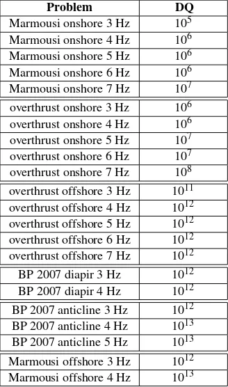
Borrowing a device from the numerical optimization literature, we measured the nonlinearity of each model/misfit combina-tion in terms of the size of the third derivatives of the misfit function (Nash and Nocedal, 1991). Because the third deriva-tives vanish if the misfit function is quadratic, the expression
DQ=kg|minit−g|mtrue−H|mtruepk∞
kpk2 ∞
, (14)
wheregis the gradient,His the Hessian andp=minit−mtrue,
provides a measure of deviation from a quadratic form. We find that the resulting ranking, shown in Table 1, agrees with our subjective sense of how easy or hard each test problem is (with the somewhat odd exception of the BP 2007 anticline test case, which has an unexpectedly high DQ).
TESTING PROCEDURES
For each model/misfit/material combination, we carried out a suite of inversions, each with the same starting model but with different frequency bands. While varying the frequency band between inversion, we kept the dominant frequency fixed within each inversion, forgoing any type of multiscale proce-dure in the manner of Bunks et al. (1995).
In these experiments, forward and adjoint simulations were carried out using SPECFEM2D, with full elastic/acoustic cou-pling for offshore problems (Komatitsch and Vilotte, 1998; Luo et al., 2013). Nonlinear optimization, data pre-processing, gradient postpre-processing, and workflow integra-tion tasks were performed in the SeisFlows framework
(http://github.com/PrincetonUniversity/seisflows). In generat-ing data and synthetics, an absorbgenerat-ing boundary condition was used to exclude multiple reflections.
To avoid problematic tradeoffs between parameters, we treated density as a dependent variable through Gardner’s relation. While such relations can be used to modify the gradient di-rectly, i.e., by substitutingδ ρ= ∂ ρ∂ κδ κ+∂ ρ∂ µδ µ in eq. 1, a more effective approach, we find, is to simply drop theKρδ ρ
term, that is, to update all parameters aside from density by their respective kernels and then, using these new values, up-date density by its empirical relation.
To avoid complicated choices about penalty function weights, we employed a simple “regularization by convolution” ap-proach in which kernels were convolved with a Gaussian with a fixed standard deviation of 5 numerical grid points, or roughly 100 m (e.g., Tape et al. 2007).
To ensure meaningful comparisons between inversion results, close attention was paid to the nonlinear optimization proce-dure. Inversions were run using L-BFGS with a memory of five previous gradient evaluations and with M3 scaling (Liu and Nocedal, 1989), stopping after convergence to a minimum of the misfit function or 100 model updates, whichever oc-curred first. For comparison, a subset of inversions was rerun using truncated Newton model updates with Eisenstat-Walker stopping condition and L-BFGS preconditioner, stopping after convergence or 50 model updates. A backtracking line search with bound constraints was used with both types of search di-rections (Dennis and Schnabel, 1996).
Numerical safeguards are important in L-BFGS inversions be-cause the accuracy of the quasi-Newton approximation to the inverse Hessian is known to break down on occasion. Besides line search bounds, restarting the nonlinear optimization algo-rithm in the manner of Powell (1977) is essential. By restart-ing when the angle between the steepest descent direction and search direction exceeds a certain threshold, say 85 degrees, we adapt Powell’s restart condition to L-BFGS. Restarting is usually effective, we find, in restoring fast convergence if an inversion becomes stalled. Details about the number of restarts in the waveform-difference (χ1) inversions are given in
Ta-ble 2. Compared with acoustic inversion, the need for restart-ing in elastic inversion is much greater.
To rate the performance of an inversion, we used the following measure of error reduction
∆E=
N X
i=1
wi kmi−1−mtruek − kmi−mtruek, (15)
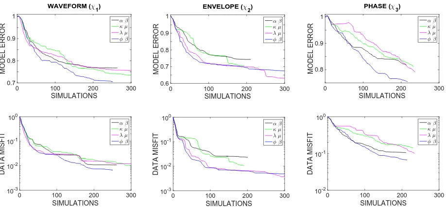
0 100 200 300
Figure 1: Model and data space convergence plots for theMarmousi onshore 3 Hztest case quasi-Newton inversions. In as far as phase misfit tends to perform well withφ,β and envelope misfit tends to perform well withλ,µ, these results are representative of
the entire suite of inversions. By “simulations” we mean the cumulative number of forward and adjoint simulations normalized by the number of sources, or equivalently, the cumulative number of function and gradient evaluations. While in this example model error closely tracks data misfit, behavior in the two spaces is not always so strongly correlated.
parameter sets toα andβ and usedkmk=kmαk2+kmβk2
in calculating∆E, wherek · k2 is theL2norm. LettingFibe
the cumulative number of function and gradient evaluations through thei-th model update, our choice of weights
wi= Fi−Fi−1)−12−0.01Fi (16)
rewards progress early in an inversion over progress later on. Such weights are important because without them eq. 15 would reduce tokm0−mtruek − kmN−mtruek. It follows that some
type of weighting is required to distinguish between two in-versions that converge to the same result at different computa-tional expense.
RESULTS
Tables 3 and 4 list which parameter sets, of the four con-sidered, performed best and worst in the quasi-Newton in-versions in terms of ∆E. Asterisks denote near ties—in which the winner came within 2.5 percent of the next-closest competitor. For illustration, convergence plots for the Mar-mousi onshore 3 Hz quasi-Newton inversions are shown in Figure 1. Plots for all other test cases are available online (http://github.com/rmodrak/SEG 2016 abstract).
In the results, strong problem dependence is evident with ma-jor differences between onshore and offshore test cases related to underlying differences in nonlinearity. Strikingly,λ andµ ranked first in more than 30 percent andαandβranked last in more than 65 percent of test cases—despite the latter’s physi-cal relevance and the former’s lack thereof. Besides poor sphysi-cal- scal-ing and large covariance betweenα andβ, much of this be-havior, we believe, can be explained in terms of relationships
between material parameters and data misfit—in particular, the fact that wave speed perturbations are more directly related to phase differences and than waveform or envelope differences.
To check whether our rankings depended strongly on any as-pect of our L-BFGS implementation, we compared quasi-Newton with truncated quasi-Newton inversion results. Truncated Newton was less computationally efficient than L-BFGS, which is not inconsistent with M´etivier et al. (2014) and not unexpected given the lack of sophisticated preconditioning (Akc¸elik et al., 2002). Although inversions based onα and β did tend to fail less often with truncated Newton model updates, rankings were not significantly affected. Leaving aside computational cost differences, the similarity between L-BFGS and truncated Newton results, in our view, suggests that robustness is more a matter of numerical safeguards than a question of one nonlinear optimization algorithm over another.
CONCLUSIONS
Problem DQ Marmousi onshore 3 Hz 105 Marmousi onshore 4 Hz 106 Marmousi onshore 5 Hz 106
Marmousi onshore 6 Hz 106 Marmousi onshore 7 Hz 107
overthrust onshore 3 Hz 106 overthrust onshore 4 Hz 106
overthrust onshore 5 Hz 107 overthrust onshore 6 Hz 107
overthrust onshore 7 Hz 108 overthrust offshore 3 Hz 1011 overthrust offshore 4 Hz 1012 overthrust offshore 5 Hz 1012 overthrust offshore 6 Hz 1012
overthrust offshore 7 Hz 1012 BP 2007 diapir 3 Hz 1012 BP 2007 diapir 4 Hz 1012 BP 2007 anticline 3 Hz 1012 BP 2007 anticline 4 Hz 1013
BP 2007 anticline 5 Hz 1013 Marmousi offshore 3 Hz 1012 Marmousi offshore 4 Hz 1013
Table 1: Deviation from quadratic. The above ranking, based on waveform-difference misfit (χ1) agrees mostly with our
subjective sense of difficulty.
Problem α,β κ,µ λ,µ φ,β
Marmousi onshore 3 Hz 4 8 10 2 Marmousi onshore 4 Hz 3 11 12 0 Marmousi onshore 5 Hz 1 7 7 0 Marmousi onshore 6 Hz 1 8 6 0 Marmousi onshore 7 Hz 0 4 5 2 overthrust onshore 3 Hz 2 6 4 1 overthrust onshore 4 Hz 3 7 7 2 overthrust onshore 5 Hz 2 6 6 2 overthrust onshore 6 Hz 1 5 7 2 overthrust onshore 7 Hz 3 6 6 4 overthrust offshore 3 Hz 2 2 4 2 overthrust offshore 4 Hz 1 3 5 2 overthrust offshore 5 Hz 1 2 2 0 overthrust offshore 6 Hz 2 3 1 2 overthrust offshore 7 Hz 0 3 4 3 BP 2007 diapir 3 Hz 0 33 7 1 BP 2007 diapir 4 Hz 2 7 8 5 BP 2007 anticline 3 Hz 0 1 1 1 BP 2007 anticline 4 Hz 1 1 1 1 BP 2007 anticline 5 Hz 1 0 0 0 Marmousi offshore 3 Hz 0 4 3 3 Marmousi offshore 4 Hz 1 5 4 0
Table 2: Number of restarts in the waveform-based (χ1)
inver-sions. A high number of restarts, we find, does not necessarily indicate a given parameterization is performing badly.
Problem Envelope Waveform Phase Marmousi onshore 3 Hz λ,µ φ,β φ,β
Marmousi onshore 4 Hz φ,β φ,β φ,β
Marmousi onshore 5 Hz φ,β φ,β —
Marmousi onshore 6 Hz φ,β φ,β —
Marmousi onshore 7 Hz φ,β φ,β —
overthrust onshore 3 Hz λ,µ λ,µ* λ,µ*
overthrust onshore 4 Hz λ,µ φ,β φ,β
overthrust onshore 5 Hz λ,µ φ,β φ,β*
overthrust onshore 6 Hz λ,µ φ,β* φ,β
overthrust onshore 7 Hz κ,µ* φ,β* φ,β*
overthrust offshore 3 Hz φ,β φ,β φ,β
overthrust offshore 4 Hz — λ,µ φ,β
overthrust offshore 5 Hz — λ,µ —
overthrust offshore 6 Hz — λ,µ —
overthrust offshore 7 Hz — λ,µ —
BP 2007 diapir 3 Hz — α,β φ,β
BP 2007 diapir 4 Hz — κ,µ —
BP 2007 anticline 3 Hz — λ,µ κ,µ
BP 2007 anticline 4 Hz — λ,µ κ,µ
BP 2007 anticline 5 Hz — λ,µ —
Marmousi offshore 3 Hz — α,β κ,µ
Marmousi offshore 4 Hz — φ,β —
Table 3: Best-performing material parameterization in terms of model error reduction (∆E). Asterisk indicates a near tie. Dash denotes all parameterizations failed.
Problem Envelope Waveform Phase Marmousi onshore 3 Hz α,β λ,µ κ,µ
Marmousi onshore 4 Hz α,β κ,µ* α,β
Marmousi onshore 5 Hz α,β α,β —
Marmousi onshore 6 Hz α,β* α,β —
Marmousi onshore 7 Hz κ,µ α,β —
overthrust onshore 3 Hz α,β φ,β α,β
overthrust onshore 4 Hz α,β α,β* α,β
overthrust onshore 5 Hz α,β α,β α,β*
overthrust onshore 6 Hz α,β α,β κ,µ
overthrust onshore 7 Hz α,β λ,µ κ,µ*
overthrust offshore 3 Hz α,β α,β α,β
overthrust offshore 4 Hz — κ,µ* α,β
overthrust offshore 5 Hz — κ,µ —
overthrust offshore 6 Hz — α,β —
overthrust offshore 7 Hz — α,β —
BP 2007 diapir 3 Hz — κ,µ α,β
BP 2007 diapir 4 Hz — λ,µ —
BP 2007 anticline 3 Hz — α,β φ,β
BP 2007 anticline 4 Hz — α,β α,β
BP 2007 anticline 5 Hz — α,β* —
Marmousi offshore 3 Hz — φ,β λ,µ
Marmousi offshore 4 Hz — α,β —
REFERENCES
Akc¸elik, A., G. Biros, and O. Ghattas, 2002, Parallel mul-tiscale Gauss-Newton-Krylov methods for inverse wave propagation.
Bozdag, E., J. Trampert, and J. Tromp, 2011, Misfit functions for full waveform inversion based on instantaneous phase and envelope measurements: Geophysical Journal Interna-tional,185, 845–870.
Bunks, C., M. Fatimetou, S. Zaleski, and G. Chavent, 1995, Multiscale seismic waveform inversion: Geophysics, 60, 1457–1473.
Cai, X.-C., and D. E. Keyes, 2002, Nonlinearly preconditioned inexact Newton algorithms: SIAM Journal on Scientific Computing,24, 183–200.
Dennis, J., and R. Schnabel, 1996, Numerical methods for un-constrained optimization and nonlinear equations: SIAM. Komatitsch, D., and J.-P. Vilotte, 1998, The spectral element
method: an efficient tool to simulate the seismic response of 2D and 3D geologic structures: Bulletin of the Seismo-logical Society of America,88, 368–392.
Liu, D., and J. Nocedal, 1989, On the limited memory BFGS method for large scale optimization: Mathematical Pro-gramming,45, 504–528.
Luo, Y., J. Tromp, B. Denel, and H. Calandra, 2013, 3d coupled acoustic-elastic migration with topography and bathymetry based on spectral-element and adjoint methods: Geophysics,78, S193–S202.
M´etivier, L., F. Bretaudeau, R. Brossier, S. Operto, and J. Virieux, 2014, Full waveform inversion and the truncated Newton method: quantitative imaging of complex subsur-face structures: Geophysical Prospecting, 1–23.
Nash, S., and J. Nocedal, 1991, A numerical study of the limited memory BFGS method and the truncated-Newton method for large scale optimization: SIAM Journal of Op-timization,1, 358–372.
Powell, M., 1977, Restart procedures for the conjugate gradi-ent method: Mathematical Programming,12, 241–254. Tape, C., Q. Liu, and J. Tromp, 2007, Finite-frequency
tomog-raphy using adjoint methodsmethodology and examples us-ing membrane surface waves: Geophysical Journal Interna-tional,168, 1105–1129.
Tarantola, A., 1986, A strategy for nonlinear elastic inversion of seismic reflection data: Geophysics,51, 1893–1903. Tromp, J., C. Tape, and Q. Liu, 2005, Seismic tomography,
ad-joint methods, time reversal and banana-doughnut kernels: Geophysical Journal International,160, 195–216.
Yuan, Y. O., F. J. Simons, and E. Bozdag, 2015, Multiscale adjoint waveform tomography for surface and body waves: Geophysics,80, R281–R302.