173
VARIABILITY OF SATELLITE-OBSERVED SEA SURFACE HEIGHT
IN THE TROPICAL INDIAN OCEAN:
COMPARISON OF EOF AND SOM ANALYSIS
Iskhaq Iskandar
1,21. Department of Physic, FMIPA, University of Sriwijaya, Inderalaya, Ogan Ilir (OI) 30662, Sumatra Selatan, Indonesia 2. NOAA/Pacific Marine Environmental Laboratory, 7600 Sand Point Way, NE, Seattle, WA, 98115
E-mail: iskhaq.iskandar@gmail.com
Abstract
Weekly sea surface height (SSH) in the tropical Indian Ocean (20°S - 20°N) was analyzed for the period of January 1993 – December 2007 using an empirical orthogonal function (EOF) and a self-organizing maps (SOM) analysis. The EOF analysis identifies four patterns and three of them are contained in the SOM patterns. The SOM, on the other hand, characterizes the sea level variability, which shows twenty-five patterns. The patterns with low (high) sea surface height anomaly (SSHA) in the southern (northern) hemisphere associated with the monsoonal winds dominate the variation in both two methods. The SOM is also able to separate typical patterns associated with the ENSO and or the Indian Ocean Dipole (IOD) events. Low SSHA occupied the western half of the basin while high SSHA loaded in the eastern basin when the La Niña event is taking place. The El Niño event is characterized by low SSHA in the northern hemisphere, along the equator and along the eastern boundary, while high SSHA in the southwestern part of the basin. The IOD event shows a dipole like pattern with low SSHA in the east and high SSHA in the west. When the IOD co-occurred with El Niño, a distinct dipole pattern is clearly observed.
Keywords: empirical orthogonal function, Indian Ocean Dipole, sea surface height, self-organizing maps, Southern Oscillation Index
1. Introduction
The Indian Ocean is unique compare to the Pacific and Atlantic Oceans. Its northern boundary is located in the tropics and blocked by Asian landmass. One consequence of this geography is that the surface winds experience a dramatic seasonal change due to varying land-ocean temperature contrasts. These strong winds forced surface ocean circulations that modulate the evolution of sea surface temperature (SST) [1]. In addition, the Indian Ocean also receives heats from the Pacific Ocean through the Indonesian throughflow (ITF) [2] and exporting heats to the Atlantic Ocean via the Agulhas current [3].
Over the equator within a zonal band of few degrees, strong westerly winds blow during the transition period between the two monsoons in April-May and October- November. As consequence of these distinct wind patterns, the swift eastward upper ocean currents, known as the Wyrtki jet, are observed during these periods [4]. It is widely accepted that the jet plays an important role on the zonal redistribution of water mass, heat, and salt, which in turn modify SST of the warm
water pool in the eastern equatorial Indian Ocean. A slight change in the SST there results in a large variations of the air-sea interactions, thus affecting the regional and global climate system through the atmospheric teleconnections.
Due to a limited in situ data, study on the dynamics as well as thermodynamics of the Indian Ocean is far behind those in the other two oceans. Most of previous observational efforts only conducted sporadically and did not leave a significant legacy of sustained ocean observation in this peculiar ocean.
Recent discovery of an inherent coupled ocean-atmosphere phenomenon in the tropical Indian Ocean, so-called Indian Ocean Dipole (IOD), however, has been considered as a stimulated interest of the study in the Indian Ocean [5,6]. Moreover, progress in satellite observations has provided continuous and nearly global surface ocean data, such as sea surface height (SSH), SST, sea level pressure (SLP), and surface winds.
Organizing Map (SOM), analysis have been applied to the merged satellite-retrieved SSH in the tropical Indian Ocean to elucidate characteristics of its spatial as well as temporal variations. More information on the data and analysis method is given in the following section. Main finding of the saptio-temporal variations of the SSH is described in section 3. Special attention is paid to the interannual variations of the SSH and their relation with IOD and El Niño Southern Oscillation (ENSO). Summary and discussion are presented in the last section.
2. Methods
Data. The SSH data used in this study were derived from the weekly merged data from multi-satellite sensors (TOPEX/Poseidon, ERS and Jason) over the 15-year period from January 1993 to December 2007. The data have spatial resolution of 1/3° and are available at http://www.aviso.oceanobs.com
In order to reduce the impact of the seasonal cycle on the data analysis, the SSH Anomaly (SSHA) is generated by subtracting both the temporal mean map and the spatial mean SSH time series from the original dataset. Assume that the dataset is arranged in a m×n
matrix, where m is the spatial dimension and n is the temporal dimension, then the temporal mean SSH is calculated as
This temporal mean is removed from the original dataset following
The time series of spatial mean SSH is, then, obtained by
Finally, we obtained the SSHA field by removing both temporal and spatial mean from the original SSH data as
)
Empirical Orthogonal Functions (EOF). The EOF method is a useful technique for analyzing the variability of time series data [7]. The method finds the spatial patterns of variability, their temporal variations, and gives a measure of the importance of each pattern. Typically, the lowest mode explains much of the variance and these spatial and temporal patterns will be easiest to interpret.
The EOF analysis uses a set of orthogonal functions to represent a time series of spatial pattern, such that
∑
where T(x,t) is the original time series as a functionof time (t) and space (x). Fn(x) is a dimensional spatial
pattern of the major factor that can account for the temporal variations of the original time series, and αn(t)
is a nondimensional principal component that describes how the amplitude of each spatial pattern varies with time.
Self-Organizing Maps (SOM)’ The SOM is one type of unsupervised Artificial Neural Network (ANN) that is mainly used for pattern recognition and classification [8]. It is a nonlinear, ordered, smooth mapping of high-dimensional input data onto the elements of regular, low-dimensional array. The SOM has been applied widely to climate and meteorology [9,10] and oceanography [11-15]. All these studies suggested that the SOM is a powerful tool for identifying patterns of continuous, dynamic processes in complex data sets.
Since the SOM is relatively new to oceanography, a brief description of the method is discussed here. Prior to the analysis, the input data are arranged into two-dimensional array with dimensions equal to number of pixels per time step ×number of time steps.The SOM algorithm is then initiated by defining the shape and dimension of the SOM array, which depends on the complexity of the studied problem and the level of details desired in the analysis. Each node in the SOM array is associated with a weight vector wi
v
that is equal in dimension to the input vector
x
v
. Prior to the training process, the weight vectors are assigned with starting values, which can be chosen to be random values.The training process starts by presenting the first input vector to the SOM, and the activation of each unit for the presented input vector is calculated using an activation function. Here, the minimum Euclidian distance criterion is used as the activation function. The node responding maximally to a given input vector (i.e. the smallest Euclidian distance) is selected to be the “winner” ck:
i k
k x w
c =arg min r −v (6)
where “arg” denotes index,
x
kv
indicates the present input vector andwi
v
where α0 is the initial learning rate and T signifies the
length of training.
The weight vectors of units in the neighborhood of the
winner are also modified according to a spatial-temporal neighborhood function ε. The neighborhood function ε also shrinks over time and decreases spatially away from the winner. There are two types of the neighborhood function available in the software; bubble
and Gaussian functions. In this study, a bubble function is used for the neighborhood function:
) (
)
(t =Fσt−dci
ε (8)
where σtis the neighborhood radius that also linearly
decreases between the initial and the final step, dci is the
distance between a node and the winner node. F is a step function and it is defined as:
⎩
The learning rule, then, is defined as:
{
() ()}
where t denotes the current learning iteration and
x
v
indicates the currently presented input vector.The training is performed in two phases. The first phase had a learning rate of 0.5, an initial update radius of 4 and a training length of 4000 cycles. Then, the second phase had a learning rate of 0.1, an initial update radius of 1 and a training length of 100,000 cycles. At the end of the training processes, a SOM array is obtained which consists of a number of patterns characteristic of the input data, with similar patterns nearby and dissimilar patterns further apart. Several dimensions of the SOM array have been tested to find the most sufficient array that covers the original data space. It is found that a 5 × 5 SOM array is sufficient to describe the SSH variability in the tropical Indian Ocean.
Pre-processing of the data has been done before performing SOM analysis. The SHHA data have been regridded by calculating average in 2° × 2° boxes from 30°E to 120°E and 20°S to 20°N. The land was removed from the analysis, so that the input data consists of 808 sea pixels. The final input matrix consists of 808 columns (pixels) × 783 rows (weeks).
3. Results and Discussion
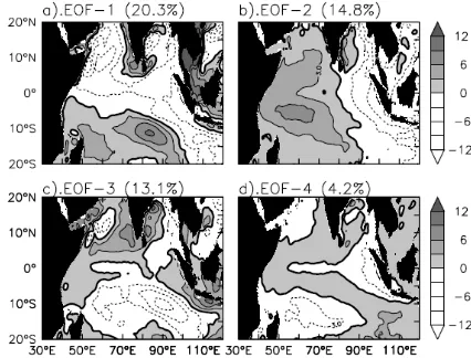
EOF results. The results from EOF analysis indicate that the first EOF mode spatial pattern, which represents 20.3% of the total variance, consists of large negative SSHA off equator along 5°S and 5°N, in the western
Arabian Sea and moderately large negative SSHA along the equator (Fig. 1a). Positive SSHA observed in the central-south and southwestern basin is considered as downwelling mid-latitude Rossby waves emanating from the eastern Indonesian and Australian coasts [16, 17].
The second EOF mode explaining 14.8% of the total variance represents a dipole pattern, with negative SSHA in the east and positive SSHA covers the western half of the basin (Fig. 1b). The spatial pattern of the third EOF mode, which accounts for 13.1% of the total variance, is a mirror of that of the first mode. Extremely low SSHA is found along 10°S, while positive SSHA is observed along the equator, off Sumatra and Java and along the coast of the Indian Peninsula (Fig. 1c).
The fourth mode, on the other hand, explains 4.2% of the total variance (Fig. 1d). The spatial structure associated with this mode shows a typical pattern of equatorial waves: Kelvin and Rossby waves. The negative SSHA associated with the upwelling equatorial Kelvin waves along the equator is accompanied by a saddle-formed of positive SSHA; north and south of the equator; indicative of a typical structure of the downwelling Rossby waves.
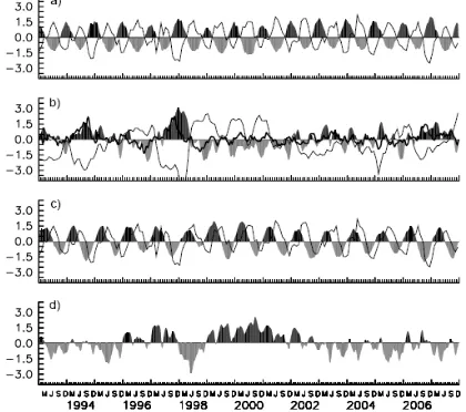
The corresponding time series (Principal component – PC) of each mode are shown in Figure 2, together with the time series of zonal wind index, Southern Oscillation Index (SOI) and Dipole Mode Index (DMI). Note that the SOI is calculated as a difference in surface air pressure between Tahiti, French Polynesia minus Darwin, Australia [18]. Its positive (negative) value is associated with La Niña (El Niño) phase of ENSO. The DMI, on the other hand, is the east-west temperature gradient across the tropical Indian Ocean [5]. Positive
DMI refers to positive IOD event, while negative IOD event is represented by negative DMI.
The time series of the first (Fig. 2a) and the third (Fig. 2c) modes exhibit a robust annual signal. This annual variation is associated with the monsoonal wind indicated by large correlation between the PCs and the zonal wind index. Note that the correlation coefficient between the PC1 (PC3) and the zonal wind index is -0.89 (-0.78; the zonal wind index leads by ~3 months) and both are significant at the 99% level.
The time series of the second mode (PC2), on the other hand, reveals interannual variation (Fig. 2b). The positive peaks occurred in 1994, 1997/98 and 2006, while the negative peaks were observed during 1996, 1998/99 and 1999-2000. The correlation between the PC2 and the SOI is -0.62 (significant at the 99% level) with the SOI leading by ~4 months. The PC2 also has significant correlation (0.45 - significant at the 99% level) with the DMI. The high correlation between the PC2 and both SOI and DMI suggests that both ENSO and IOD events contribute to the interannual variation of the SSHA in the tropical Indian Ocean. This result is consistent with the early studies in the tropical Indian Ocean [5, 19].
The time series of the fourth mode (PC4) reveals long-lasting positive peaks occurring during 1999-2001, and strong negative peaks during 1995, 1998 and 2005. The
Figure 2. Time Series (Black-Gray Shade) Corresponding to the Modes on Figure 1. Thin-Curve in (a) and (c) is Time Series of Zonal Wind Average between 40°E-100°E and 5°S-5°N. Thin (Thick) Curve in (b) is Southern Oscillation Index (Dipole Mode Index)
correlation between the PC4 and the SOI is 0.6 (significant at the 99% level) with the SOI leading by ~7 months. However, the PC4 has no significant correlation with the DMI, which may suggest that the variation of PC4 is solely associated with the ENSO.
SOM results. The SOM array that obtained from the observed sea surface height is shown in Fig. 3. The array consists of 25 nodes, where each node represents a typical structure of the input data. Frequencies of occurrence of each SOM node are shown in the above of each node. The lower-right corner of the array is populated by low SSHA in the southern hemisphere while high SSHA in the northern hemisphere, along the equator and along the coast of Sumatra and Java. These nodes (i.e. nodes 15, 19, 20, 23, 24 and 25) are the most common patterns throughout the whole record representing 30.1% occurrence. The spatial pattern of these modes is very similar to that of the first mode from EOF analysis, and they are major patterns in each method.
Conversely, the center-left corner (nodes 7, 8, 11, 12, 16 and 21) shows high SSHA in the south and low SSHA in the north, which are compatible with the third mode of EOF analysis. These patterns are accounting for 15.5% of occurrence.
In the center of the array (nodes 9, 13, 14, 17, 18, 21, and 22), the patterns show a dipole structure with low SSHA in the east and high SSHA in the west. Note that the spatial structures of the nodes 13 and 14 are very much compatible with that of the second mode of the EOF analysis. The nodes reflect 22.7% of the occurrence. On the other hand, the upper-left corner (nodes 1, 2 and 6) shows opposite structure, with high SSHA in the east and low SSHA in the west.
The upper-right corner (node 3, 4, 7, 8, 11 and 12) represents low SSHA in the south and along the eastern boundary, while high SSHA in the northwestern part of the basin. However, these nodes have no counterparts in the EOF modes. Similarly, the fourth mode of EOF resu lts does no t appear in t h e SO M patterns.
Figure 3. A 5 × 5 SOM Representation of the SSHA Time Series from January 1993 trough December 2007. The Frequency of Occurrence is Shown Above Each Panel
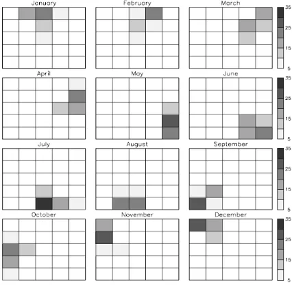
Figure 4. Monthly Frequency Map, Showing the Frequency that SOM Patterns Identified in Fig. 3 Occurred for Each Month. Note that Percentage for Each Month Sum to 100 and the Coordinates Correspond to those at Fig. 3
To examine the interannual variations in SSHA, a relative frequency map was constructed for some contrasting years, which are identified as the ENSO and or the IOD years. Figure 5 shows the annual frequency maps during La Niña, El Niño, IOD and El Niño co-occurring with IOD events. Note that for the El Niño and La Niña events, the frequency maps were calculated from September to February of the following year to encompass the peak of the events. On the other hand, the frequency maps for the IOD event were constructed from June to November, since the peak of the IOD event is during the northern fall (i.e. September to October).
Figure 5. Annual Frequency Map, Showing How Many Time Each Particular Node in the SOM Array Appear During Each Event: ENSO and IOD
During La Niña event, on the other hand, the node 1 dominates the variations, which represent positive SSHA in the east while negative SSHA is observed in the western basin, showing opposite pattern to that of the IOD event. The mechanism generating this pattern is also opposite to that of the IOD event.
The El Niño event is mostly dominated by node 7 showing negative SSHA in the northern part, along the equator and along the eastern boundary, and positive SSHA in the southwestern part of the basin. The mechanism generating this pattern is similar to that of the IOD pattern.
Interestingly, during 1997/98 when the IOD and El Niño took place in the Indian Ocean, node 13 dominated the pattern, which indicates a robust dipole pattern with low SSHA in the east and high SSHA in the west.
Spatial and temporal variations of SSHA in the tropical Indian Ocean are examined with the EOF and SOM analysis. The EOF analysis identified only four patterns, in which three of them are included in the SOM array. The first and the third modes of the EOF accounting for 33.4% of the total variance explain much of the variability in the tropical Indian Ocean. This variation is associated with the monsoonal winds, which vary annually. The second mode of the EOF, on the other hand, explains 14.8% of the total variance. This mode showing a dipole structure is significantly correlated with the ENSO and the IOD events. The fourth mode only explains 4.2% of the total variance and it is likely related to the ENSO variation.
A 5 × 5 SOM array also shows characteristic sea level patterns. These group into three composite categories: a pattern with low (high) SSHA in the southern (northern) hemisphere, a dipole pattern and a pattern with low SSHA in the southern hemisphere and along the eastern boundaries, while high SSHA is observed in the northwestern basin.
A significant finding identified herein by the SOM, and not by the EOF, is that the patterns of sea level variability associated with the ENSO and or the IOD events. The pattern associated with the La Niña event is characterized by low SSHA in the west and high SSHA in the east. The El Niño event is characterized by low SSHA in the northern hemisphere, along the equator and along the eastern boundary, while high SSHA in the southwestern part of the basin. The IOD event shows a dipole like pattern with low SSHA in the east and high SSHA in the west. In 1997/98 when the IOD and El Niño events took place in the tropical Indian Ocean, a distinct dipole pattern is observed with low SSHA in the eastern half of the basin and high SSHA occupied the western half of the basin.
4. Conclusion
The use of the SOM to characterize the sea level patterns in the tropical Indian Ocean has provided a clear description of the main sea level patterns associated with the monsoon, ENSO and IOD. From this point of view, the (nonlinear) SOM is more convenient to use than the (linear) EOF.
Acknowledgment
The gridded sea surface height data are from Live Access server of AVISO user service (http://www.aviso.oceanobs. com). The SOM_PAK was prepared by the SOM Programming Team of the Helsinki University of Technology, Finland. The author is grateful for the support from the Japan Society for the Promotion of Science through the Postdoctoral Fellowships for Foreign Researcher.
References
[1] F.A., Schott, J.P. McCreary, Prog. Oceanogr. 51 (2001), 1-123.
[2] A.L. Gordon, In: G. Siedler, J. Church, J. Gould (Eds.), Ocean Circulation and Climate, Academic Press, New York, 2001, pp. 303-314.
[3] W.P.M. de Ruijter, A. Biastoch, S.S. Drijfhourt, J.R.E. Lutjeharms, R.P. Matano, T. Pichevin, P.J. van Leeuwen, W. Weijer, J. Geophys. Res., 29 (1999) 1166-1184.
[5] N.H. Saji, B.N. Goswami, P.N. Vinayachandran, T. Yamagata, Nature, 401 (1999) 360-363.
[6] P.J. Webster, A.M. Moore, J.P. Loschnigg, R.R. Leben, Nature, 401 (1999) 356-359.
[7] W.J. Emery, R.E. Thomson, Data Analysis Methods in Physical Oceanography, 2nd ed., Elseiver, Amsterdam, 2001, p. 638.
[8] T. Kohonen, Self-Organizing Maps, 3rd ed., Springer-Verlag Berlin, Heidelberg, New York, 2001, p. 501.
[9] B.C. Hewitson, R.G. Crane, Clim. Res., 22 (2002) 13-26.
[10] T. Cavazos, J. Climate, 13 (2000) 1718-1732. [11] A.J. Richardson, C. Risien, F.A. Shillington, Prog.
Oceanogr., 59 (2003) 223-239.
[12] Y. Liu, R.H. Weisberg, J. Geophys. Res., 110 (2005) C06003, doi:10.1029/2004JC002786.
[13] Y. Liu, R.H. Wesiberg, R. He, J. Atmos. Oceanic Technol., 23 (2006) 235-338.
[14] P. Cheng, R.E. Wilson, J. Geophys. Res., 111 (2006) C12021, doi:10.1029/2005JC003241. [15] I. Iskandar, T. Tozuka, Y. Masumoto, T.
Yamagata, Geophys. Res. Lett., 35, L14S03 (2008) doi:10.1029/ 2008GL033468.
[16] J.T. Potemra, R. Lukas, Geophys. Res. Lett., 26 (1999) 365-368.
[17] S.A. Rao, S.K. Behera, Y. Masumoto, T. Yamagata, Deep Sea Res. II, 49 (2002) 1549-1572. [18] M.J. McPhaden, Bull. American Meteor. Soc., 85
(2004) 677-695.