Marvin K. Simon, Mohamed-Slim Alouini Copyright2000 John Wiley & Sons, Inc. Print ISBN 0-471-31779-9 Electronic ISBN 0-471-20069-7
Digital Communication
over Fading Channels
Digital Communication
over Fading Channels
A Unified Approach
to Performance Analysis
Marvin K. Simon
Mohamed-Slim Alouini
all instances where John Wiley & Sons, Inc., is aware of a claim, the product names appear in initial capital or ALL CAPITAL LETTERS. Readers, however, should contact the appropriate companies for more complete information regarding trademarks and registration.
Copyright2000 by John Wiley & Sons, Inc. All rights reserved.
No part of this publication may be reproduced, stored in a retrieval system or transmitted in any form or by any means, electronic or mechanical, including uploading, downloading, printing, decompiling, recording or otherwise, except as permitted under Sections 107 or 108 of the 1976 United States Copyright Act, without the prior written permission of the Publisher. Requests to the Publisher for permission should be addressed to the Permissions Department, John Wiley & Sons, Inc., 605 Third Avenue, New York, NY 10158-0012, (212) 850-6011, fax (212) 850-6008, E-Mail: [email protected].
This publication is designed to provide accurate and authoritative information in regard to the subject matter covered. It is sold with the understanding that the publisher is not engaged in rendering professional services. If professional advice or other expert assistance is required, the services of a competent professional person should be sought.
ISBN 0-471-20069-7.
This title is also available in print as ISBN 0-471-31779-9.
For more information about Wiley products, visit our web site at www.Wiley.com. Library of Congress Cataloging-in-Publication Data:
Simon, Marvin Kenneth, 1939–
Digital communication over fading channels : a unified approach to performance analysis / Marvin K. Simon and Mohamed-Slim Alouini.
p. cm. — (Wiley series in telecommunications and signal processing) Includes index.
ISBN 0-471-31779-9 (alk. paper)
1. Digital communications — Reliability — Mathematics. I. Alouini, Mohamed-Slim. II. Title. III. Series.
TK5103.7.S523 2000
621.382 — dc21 99-056352
whose devotion to him and this project never once faded during its preparation. Mohamed-Slim Alouini dedicates this book
Marvin K. Simon, Mohamed-Slim Alouini Copyright2000 John Wiley & Sons, Inc. Print ISBN 0-471-31779-9 Electronic ISBN 0-471-20069-7
CONTENTS
Preface xv
PART 1 FUNDAMENTALS
Chapter 1 Introduction 3
1.1 System Performance Measures 4
1.1.1 Average Signal-to-Noise Ratio 4
1.1.2 Outage Probability 5
1.1.3 Average Bit Error Probability 6
1.2 Conclusions 12
References 13
Chapter 2 Fading Channel Characterization and Modeling 15
2.1 Main Characteristics of Fading Channels 15
2.1.1 Envelope and Phase Fluctuations 15
2.1.2 Slow and Fast Fading 16
2.1.3 Frequency-Flat and Frequency-Selective
Fading 16
2.2 Modeling of Flat Fading Channels 17
2.2.1 Multipath Fading 18
2.2.2 Log-Normal Shadowing 23
2.2.3 Composite Multipath/Shadowing 24
2.2.4 Combined (Time-Shared)
Shadowed/Unshadowed Fading 25
2.3 Modeling of Frequency-Selective Fading
Channels 26
References 28
Chapter 3 Types of Communication 31
3.1 Ideal Coherent Detection 31
3.1.1 Multiple Amplitude-Shift-Keying or
Multiple Amplitude Modulation 33
3.1.2 Quadrature Amplitude-Shift-Keying or
Quadrature Amplitude Modulation 34
3.1.3 M-ary Phase-Shift-Keying 35
3.1.4 Differentially EncodedM-ary
Phase-Shift-Keying 39
3.1.5 Offset QPSK or Staggered QPSK 41
3.1.6 M-ary Frequency-Shift-Keying 43
3.1.7 Minimum-Shift-Keying 45
3.2 Nonideal Coherent Detection 47
3.3 Noncoherent Detection 53
3.4 Partially Coherent Detection 55
3.4.1 Conventional Detection: One-Symbol
Observation 55
3.4.2 Multiple Symbol Detection 57
3.5 Differentially Coherent Detection 59
3.5.1 M-ary Differential Phase Shift Keying 59
3.5.2 /4-Differential QPSK 65
References 65
PART 2 MATHEMATICAL TOOLS
Chapter 4 Alternative Representations of Classical
Functions 69
4.1 Gaussian Q-Function 70
4.1.1 One-Dimensional Case 70
4.1.2 Two-Dimensional Case 72
4.2 MarcumQ-Function 74
4.2.1 First-Order MarcumQ-Function 74
4.2.2 Generalized (mth-Order) Marcum
Q-Function 81
4.3 Other Functions 90
References 94
Appendix 4A: Derivation of Eq. (4.2) 95
Chapter 5 Useful Expressions for Evaluating Average Error
Probability Performance 99
5.1 Integrals Involving the Gaussian Q-Function 99
5.1.2 Nakagami-q(Hoyt) Fading Channel 101
5.1.3 Nakagami-n(Rice) Fading Channel 102
5.1.4 Nakagami-mFading Channel 102
5.1.5 Log-Normal Shadowing Channel 104
5.1.6 Composite Log-Normal
Shadowing/Nakagami-m Fading Channel 104
5.2 Integrals Involving the Marcum Q-Function 107
5.2.1 Rayleigh Fading Channel 108
5.2.2 Nakagami-q(Hoyt) Fading Channel 109
5.2.3 Nakagami-n(Rice) Fading Channel 109
5.2.4 Nakagami-mFading Channel 109
5.2.5 Log-Normal Shadowing Channel 109
5.2.6 Composite Log-Normal
Shadowing/Nakagami-m Fading Channel 110 5.3 Integrals Involving the Incomplete Gamma
Function 111
5.3.1 Rayleigh Fading Channel 112
5.3.2 Nakagami-q(Hoyt) Fading Channel 112
5.3.3 Nakagami-n(Rice) Fading Channel 112
5.3.4 Nakagami-mFading Channel 113
5.3.5 Log-Normal Shadowing Channel 114
5.3.6 Composite Log-Normal
Shadowing/Nakagami-m Fading Channel 114
5.4 Integrals Involving Other Functions 114
5.4.1 M-PSK Error Probability Integral 114
5.4.2 Arbitrary Two-Dimensional Signal
Constellation Error Probability Integral 116 5.4.3 Integer Powers of the Gaussian
Q-Function 117
5.4.4 Integer Powers of M-PSK Error
Probability Integrals 121
References 124
Appendix 5A: Evaluation of Definite Integrals
Associated with Rayleigh and Nakagami-mFading 124
Chapter 6 New Representations of Some PDF’s and CDF’s
for Correlative Fading Applications 141
6.1 Bivariate Rayleigh PDF and CDF 142
6.2 PDF and CDF for Maximum of Two Rayleigh
Random Variables 146
6.3 PDF and CDF for Maximum of Two
Nakagami-m Random Variables 149
PART 3 OPTIMUM RECEPTION AND PERFORMANCE EVALUATION
Chapter 7 Optimum Receivers for Fading Channels 157
7.1 Case of Known Amplitudes, Phases, and Delays:
Coherent Detection 159
7.2 The Case of Known Phases and Delays,
Unknown Amplitudes 163
7.2.1 Rayleigh Fading 163
7.2.2 Nakagami-mFading 164
7.3 Case of Known Amplitudes and Delays,
Unknown Phases 166
7.4 Case of Known Delays and Unknown
Amplitudes and Phases 168
7.4.1 One-Symbol Observation: Noncoherent
Detection 168
7.4.2 Two-Symbol Observation: Conventional
Differentially Coherent Detection 181
7.4.3 N-Symbol Observation: Multiple Symbol
Differentially Coherent Detection 186
7.5 Case of Unknown Amplitudes, Phases, and
Delays 188
7.5.1 One-Symbol Observation: Noncoherent
Detection 188
7.5.2 Two-Symbol Observation: Conventional
Differentially Coherent Detection 190
References 191
Chapter 8 Performance of Single Channel Receivers 193
8.1 Performance Over the AWGN Channel 193
8.1.1 Ideal Coherent Detection 194
8.1.2 Nonideal Coherent Detection 206
8.1.3 Noncoherent Detection 209
8.1.4 Partially Coherent Detection 210
8.1.5 Differentially Coherent Detection 213
8.1.6 Generic Results for Binary Signaling 218
8.2 Performance Over Fading Channels 219
8.2.1 Ideal Coherent Detection 220
8.2.2 Nonideal Coherent Detection 234
8.2.3 Noncoherent Detection 239
8.2.4 Partially Coherent Detection 242
8.2.5 Differentially Coherent Detection 243
Appendix 8A: Stein’s Unified Analysis of the Error Probability Performance of Certain Communication
Systems 253
Chapter 9 Performance of Multichannel Receivers 259
9.1 Diversity Combining 260
9.1.1 Diversity Concept 260
9.1.2 Mathematical Modeling 260
9.1.3 Brief Survey of Diversity Combining
Techniques 261
9.1.4 Complexity–Performance Trade-offs 264
9.2 Maximal-Ratio Combining 265
9.2.1 Receiver Structure 265
9.2.2 PDF-Based Approach 267
9.2.3 MGF-Based Approach 268
9.2.4 Bounds and Asymptotic SER
Expressions 275
9.3 Coherent Equal Gain Combining 278
9.3.1 Receiver Structure 279
9.3.2 Average Output SNR 279
9.3.3 Exact Error Rate Analysis 281
9.3.4 Approximate Error Rate Analysis 288
9.3.5 Asymptotic Error Rate Analysis 289
9.4 Noncoherent Equal-Gain Combining 290
9.4.1 DPSK, DQPSK, and BFSK: Exact and
Bounds 290
9.4.2 M-ary Orthogonal FSK 304
9.5 Outage Probability Performance 311
9.5.1 MRC and Noncoherent EGC 312
9.5.2 Coherent EGC 313
9.5.3 Numerical Examples 314
9.6 Impact of Fading Correlation 316
9.6.1 Model A: Two Correlated Branches with
Nonidentical Fading 320
9.6.2 Model B:DIdentically Distributed
Branches with Constant Correlation 323
9.6.3 Model C:DIdentically Distributed
Branches with Exponential Correlation 324 9.6.4 Model D: DNonidentically Distributed
Branches with Arbitrary Correlation 325
9.6.5 Numerical Examples 329
9.7 Selection Combining 333
9.7.2 Average Output SNR 336
9.7.3 Outage Probability 338
9.7.4 Average Probability of Error 340
9.8 Switched Diversity 348
9.8.1 Performance of SSC over Independent
Identically Distributed Branches 348
9.8.2 Effect of Branch Unbalance 362
9.8.3 Effect of Branch Correlation 366
9.9 Performance in the Presence of Outdated or
Imperfect Channel Estimates 370
9.9.1 Maximal-Ratio Combining 370
9.9.2 Noncoherent EGC over Rician Fast
Fading 371
9.9.3 Selection Combining 373
9.9.4 Switched Diversity 374
9.9.5 Numerical Results 377
9.10 Hybrid Diversity Schemes 378
9.10.1 Generalized Selection Combining 378
9.10.2 Generalized Switched Diversity 403
9.10.3 Two-Dimensional Diversity Schemes 408
References 411
Appendix 9A: Alternative Forms of the Bit Error Probability for a Decision Statistic that is a Quadratic
Form of Complex Gaussian Random Variables 421
Appendix 9B: Simple Numerical Techniques for the Inversion of the Laplace Transform of Cumulative
Distribution Functions 427
9B.1 Euler Summation-Based Technique 427
9B.2 Gauss–Chebyshev Quadrature-Based
Technique 428
Appendix 9C: Proof of Theorem 1 430
Appendix 9D: Direct Proof of Eq. (9.331) 431
Appendix 9E: Special Definite Integrals 432
PART 4 APPLICATION IN PRACTICAL COMMUNICATION SYSTEMS
Chapter 10 Optimum Combining: A Diversity Technique for Communication Over Fading Channels in the
Presence of Interference 437
10.1 Performance of Optimum Combining
10.1.1 Single Interferer, Independent Identically
Distributed Fading 438
10.1.2 Multiple Interferers, Independent
Identically Distributed Fading 454
10.1.3 Comparison with Results for MRC in the
Presence of Interference 466
References 470
Chapter 11 Direct-Sequence Code-Division Multiple Access 473
11.1 Single-Carrier DS-CDMA Systems 474
11.1.1 System and Channel Models 474
11.1.2 Performance Analysis 477
11.2 Multicarrier DS-CDMA Systems 479
11.2.1 System and Channel Models 480
11.2.2 Performance Analysis 483
11.2.3 Numerical Examples 489
References 492
PART 5 FURTHER EXTENSIONS
Chapter 12 Coded Communication Over Fading Channels 497
12.1 Coherent Detection 499
12.1.1 System Model 499
12.1.2 Evaluation of Pairwise Error Probability 502 12.1.3 Transfer Function Bound on Average Bit
Error Probability 510
12.1.4 Alternative Formulation of the Transfer
Function Bound 513
12.1.5 Example 514
12.2 Differentially Coherent Detection 520
12.2.1 System Model 520
12.2.2 Performance Evaluation 522
12.2.3 Example 524
12.3 Numerical Results: Comparison of the True
Upper Bounds and Union–Chernoff Bounds 526
References 530
Appendix 12A: Evaluation of a Moment Generating Function Associated with Differential Detection of
M-PSK Sequences 532
Marvin K. Simon, Mohamed-Slim Alouini Copyright2000 John Wiley & Sons, Inc. Print ISBN 0-471-31779-9 Electronic ISBN 0-471-20069-7
PREFACE
Regardless of the branch of science or engineering, theoreticians have always been enamored with the notion of expressing their results in the form of closed-form expressions. Quite often, the elegance of the closed-form solution is overshadowed by the complexity of its form and the difficulty in evaluating it numerically. In such instances, one becomes motivated to search instead for a solution that is simple in form and simple to evaluate. A further motivation is that the method used to derive these alternative simple forms should also be applicable in situations where closed-form solutions are ordinarily unobtainable. The search for and ability to find such a unified approach for problems dealing with evaluation of the performance of digital communication over generalized fading channels is what provided the impetus to write this book, the result of which represents the backbone for the material contained within its pages.
For at least four decades, researchers have studied problems of this type, and system engineers have used the theoretical and numerical results reported in the literature to guide the design of their systems. Whereas the results from the earlier years dealt mainly with simple channel models (e.g., Rayleigh or Rician multipath fading), applications in more recent years have become increasingly sophisticated, thereby requiring more complex models and improved diversity techniques. Along with the complexity of the channel model comes the complexity of the analytical solution that enables one to assess performance. With the mathematical tools that were available previously, the solutions to such problems, when possible, had to be expressed in complicated mathematical form which provided little insight into the dependence of the performance on the system parameters. Surprisingly enough, not until recently had anyone demonstrated a unified approach that not only allows previously obtained complicated results to be simplified both analytically and computationally but also permits new results to be obtained for special cases that heretofore had resisted solution in a simple form. This approach, which the authors first presented to the public in a tutorial-style article that appeared in the September 1998 issue of theIEEE Proceedings, has spawned a new wave of publications on the subject that, we foresee based on the variety of applications to which it has already been applied, will continue well into the new millennium. The key to the success of the approach relies
on employing alternative representations of classic functions arising in the error probability analysis of digital communication systems (e.g., the Gaussian Q -function1 and the Marcum Q-function) in such a manner that the resulting expressions for average bit or symbol error rate are in a form that is rarely more complicated than a single integral with finite limits and an integrand composed of elementary (e.g., exponential and trigonometric) functions. By virtue of replacing the conventional forms of the above-mentioned functions by their alternative representations, the integrand will contain the moment generating function (MGF) of the instantaneous fading signal-to-noise ratio (SNR), and as such, the unified approach is referred to as theMGF-based approach.
In dealing with application of the MGF-based approach, the coverage in this book is extremely broad, in that coherent, differentially coherent, partially coherent and noncoherent communication systems are all handled, as well as a large variety of fading channel models typical of communication links of practical interest. Both single- and multichannel reception are discussed, and in the case of the latter, a large variety of diversity types are considered. For each combination of communication (modulation/detection) type, channel fading model, and diversity type, the average bit error rate (BER) and/or symbol error rate (SER) of the system is obtained and represented by an expression that is in a form that can readily be evaluated.2 All cases considered correspond to real practical channels, and in many instances the BER and SER expressions obtained can be evaluated numerically on a hand-held calculator.
In accomplishing the purpose set forth by the discussion above, the book focuses on developing a compendium of results that to a large extent are not readily available in standard textbooks on digital communications. Although some of these results can be found in the myriad of contributions that have been reported in the technical journal and conference literature, others are new and as yet unpublished. Indeed, aside from the fact that a significant number of the reference citations in this book are from 1999 publications, many others refer to papers that will appear in print in the new millennium. Whether or not published previously, the value of the results found in this book is that they are all colocated in a single publication with unified notation and, most important, a unified presentation framework that lends itself to simplicity of numerical evaluation. In writing this book, our intent was to spend as little space as possible duplicating material dealing with basic digital communication theory and system performance evaluation, which is well documented in many fine textbooks on the subject. Rather, this book serves to advance the material found in these books and so is of most value to those desiring to extend their knowledge
1The GaussianQ-function has a one-to-one mapping with the complementary error function erfcx [i.e.,Q⊲x⊳D12erfc⊲x/
p
2⊳] commonly found in standard mathematical tabulations. In much of the engineering literature, however, the two functions are used interchangeably and as a matter of convenience we shall do the same in this text.
beyond what ordinarily might be covered in the classroom. In this regard, the book should have a strong appeal to graduate students doing research in the field of digital communications over fading channels as well as to practicing engineers who are responsible for the design and performance evaluation of such systems. With regard to the latter, the book contains copious numerical evaluations that are illustrated in the form of parametric performance curves (e.g., average error probability versus average SNR). The applications chosen for the numerical illustrations correspond to real practical channels, therefore the performance curves provided will have far more than academic value. The availability of such a large collection of system performance curves in a single compilation allows the researcher or system designer to perform trade-off studies among the various communication type/fading channel/diversity combinations so as to determine the optimum choice in the face of his or her available constraints. The book is composed of four parts, each with an express purpose. The first part contains an introduction to the subject of communication system performance evaluation followed by discussions of the various types of fading channel models and modulation/detection schemes that together form the overall system. Part 2 starts by introducing the alternative forms of the classic functions mentioned above and then proceeds to show how these forms can be used to (1) evaluate certain integrals characteristic of communication system error probability performance, and (2) find new representations for certain probability density and distribution functions typical of correlated fading applications. Part 3 is the “heart and soul” of the book, since in keeping with its title, the primary focus of this part is on performance evaluation of the various types of fading channel models and modulation/detection schemes introduced in Part 1 for both single- and multichannel (diversity) reception. Before presenting this comprehensive performance evaluation study, however, Part 3 begins by deriving the optimum receiver structures corresponding to a variety of combinations concerning the knowledge or lack thereof of the fading parameters (i.e., amplitude, phase, delay). Several of these structures might be deemed as too complex to implement in practice; nevertheless, their performances serve as benchmarks against which many suboptimum but practical structures discussed in the ensuing chapters might be compared. In Part 4, which deals with practical applications, we consider first the problem of optimum combining (diversity) in the presence of co-channel interference and then apply the unified approach to studying the performance of single- and multiple-carrier direct-sequence code-division multiple-access (DS-CDMA) systems typical of the current digital cellular wireless standard. Finally, in Part 5 we extend the theory developed in the preceding parts for uncoded communication to error-correction-coded systems.
quarter of a century old. Although a number of other textbooks [3–11] devote part of their contents3 to fading channel performance evaluation, by comparison with our book the treatment is brief and therefore incomplete. In view of the above, we believe that our book is unique in the field.
By way of acknowledgment, we wish to thank Dr. Payman Arabshahi of the Jet Propulsion Laboratory, Pasadena, CA for providing his expertise in solving a variey of problems that arose during the preparation of the electronic version of the manuscript. Mohamed-Slim Alouini would also like to express his sincere acknowledgment and gratitude to his PhD advisor Prof. Andrea J. Goldsmith of Stanford University, Palo Alto, CA for her guidance, support, and constant encouragement. Some of the material presented in Chapters 9 and 11 is the result of joint work with Prof. Goldsmith. Mohamed-Slim Alouini would also like to thank Young-Chai Ko and Yan Xin of the University of Minnesota, Minneapolis, MN for their significant contributions in some of the results presented in Chapters 9 and 7, respectively.
MARVIN K. SIMON MOHAMED-SLIMALOUINI
Jet Propulsion Laboratory Pasadena, California University of Minnesota Minneapolis, Minnesota
REFERENCES
1. R. S. Kennedy, Fading Dispersive Communication Channels. New York: Wiley-Interscience, 1969.
2. K. Brayer, ed., Data Communications via Fading Channels. Piscataway, NJ: IEEE Press, 1975.
3. M. Schwartz, W. R. Bennett, and S. Stein,Communication Systems and Techniques. New York: McGraw-Hill, 1966.
4. W. C. Y. Lee,Mobile Communications Engineering. New York: McGraw-Hill, 1982. 5. J. Proakis,Digital Communications. New York: McGraw-Hill, 3rd ed., 1995 (1st and
2nd eds. in 1983, 1989, respectively).
6. M. D. Yacoub, Foundations of Mobile Radio Engineering. Boca Raton, FL: CRC Press, 1993.
7. W. C. Jakes, Microwave Mobile Communication, 2nd ed., Piscataway, NJ: IEEE Press, 1994.
8. K. Pahlavan and A. H. Levesque, Wireless Information Networks. Wiley Series in Telecommunications and Signal Processing. New York: Wiley-Interscience, 1995. 9. G. L. St¨uber,Principles of Mobile Communication. Norwell, MA: Kluwer Academic
Publishers, 1996.
10. T. S. Rappaport,Wireless Communications: Principles and Practice. Upper Saddle River, NJ: Prentice Hall, 1996.
Marvin K. Simon, Mohamed-Slim Alouini Copyright2000 John Wiley & Sons, Inc. Print ISBN 0-471-31779-9 Electronic ISBN 0-471-20069-7
P
ART
1
Marvin K. Simon, Mohamed-Slim Alouini Copyright2000 John Wiley & Sons, Inc. Print ISBN 0-471-31779-9 Electronic ISBN 0-471-20069-7
1
INTRODUCTION
As we step forward into the new millennium with wireless technologies leading the way in which we communicate, it becomes increasingly clear that the dominant consideration in the design of systems employing such technologies will be their ability to perform with adequate margin over a channel perturbed by a host of impairments not the least of which is multipath fading. This is not to imply that multipath fading channels are something new to be reckoned with, indeed they have plagued many a system designer for well over 40 years, but rather, to serve as a motivation for their ever-increasing significance in the years to come. At the same time, we do not in any way wish to diminish the importance of the fading channel scenarios that occurred well prior to the wireless revolution, since indeed many of them still exist and will continue to exist in the future. In fact, it is safe to say that whatever means are developed for dealing with the more sophisticated wireless application will no doubt also be useful for dealing with the less complicated fading environments of the past.
With the above in mind, what better opportunity is there than now to write a comprehensive book that provides simple and intuitive solutions to problems dealing with communication system performance evaluation over fading channels? Indeed, as mentioned in the preface, the primary goal of this book is to present a unified method for arriving at a set of tools that will allow the system designer to compute the performance of a host of different digital communication systems characterized by a variety of modulation/detection types and fading channel models. By set of tools we mean a compendium of analytical results that not only allow easy, yet accurate performance evaluation but at the same time provide insight into the manner in which this performance depends on the key system parameters. To emphasize what was stated above, the set of tools developed in this book are useful not only for the wireless applications that are rapidly filling our current technical journals but also to a host of others, involving satellite, terrestrial, and maritime communications.
Our repetitive use of the word performance thus far brings us to the purpose of this introductory chapter: to provide several measures of performance related to practical communication system design and to begin exploring the analytical
methods by which they may be evaluated. While the deeper meaning of these measures will be truly understood only after their more formal definitions are presented in the chapters that follow, the introduction of these terms here serves to illustrate the various possibilities that exist, depending on both need and relative ease of evaluation.
1.1 SYSTEM PERFORMANCE MEASURES
1.1.1 Average Signal-to-Noise Ratio
Probably the most common and best understood performance measure charac-teristic of a digital communication system is signal-to-noise ratio (SNR). Most often this is measured at the output of the receiver and is thus related directly to the data detection process itself. Of the several possible performance measures that exist, it is typically the easiest to evaluate and most often serves as an excel-lent indicator of the overall fidelity of the system. Although traditionally, the termnoise insignal-to-noise ratio refers to the ever-present thermal noise at the input to the receiver, in the context of a communication system subject to fading impairment, the more appropriate performance measure isaverage SNR, where the wordaverage refers to statistical averaging over the probability distribution of the fading. In simple mathematical terms, ifdenotes the instantaneous SNR [a random variable (RV)] at the receiver output, which includes the effect of fading, then
D
1
0
p⊲⊳ d ⊲1.1⊳
is the average SNR, wherep⊲⊳denotes the probability density function (PDF) of . To begin to get a feel for what we will shortly describe as a unified approach to performance evaluation, we first rewrite (1.1) in terms of the moment generating function (MGF) associated with, namely,
M⊲s⊳D
1
0
p⊲⊳esd ⊲1.2⊳
Taking the first derivative of (1.2) with respect tos and evaluating the result at sD0, we see immediately from (1.1) that
D dM⊲s⊳
ds
sD0
⊲1.3⊳
That is, the ability to evaluate the MGF of the instantaneous SNR (perhaps in closed form) allows immediate evaluation of the average SNR via a simple mathematical operation: differentiation.
(multichannel) reception known as maximal-ratio combining (MRC) (discussed in great detail in Chapter 9), the output SNR, , is expressed as a sum (combination) of the individual branch (channel) SNRs (i.e., DL
lD1l, where L denotes the number of channels combined). In addition, it is often reasonable in practice to assume that the channels are independent of each other (i.e., the RVs ljL
lD1 are themselves independent). In such instances, the
MGF M⊲s⊳ can be expressed as the product of the MGFs associated with each channel [i.e., M⊲s⊳DLlD1Ml⊲s⊳], which for a large variety of fading
channel statistical models can be computed in closed form.1 By contrast, even with the assumption of channel independence, computation of the probability density function (PDF) p⊲⊳, which requires convolution of the various PDFs
pl⊲l⊳j L
lD1 that characterize theLchannels, can still be a monumental task. Even
in the case where these individual channel PDFs are of the same functional form but are characterized by different average SNR’s, l, the evaluation of
p⊲⊳can still be quite tedious. Such is the power of the MGF-based approach; namely, it circumvents the need for finding the first-order PDF of the output SNR provided that one is interested in a performance measure that can be expressed in terms of the MGF. Of course, for the case of average SNR, the solution is extremely simple, namely, DL
lD1l, regardless of whether the channels are independent or not, and in fact, one never needs to find the MGF at all. However, for other performance measures and also the average SNR of other combining statistics [e.g., the sum of an ordered set of random variables typical of generalized selection combining (GSC) (discussed in Chapter 9)], matters are not quite this simple and the points made above for justifying an MGF-based approach are, as we shall see, especially significant.
1.1.2 Outage Probability
Another standard performance criterion characteristic of diversity systems oper-ating over fading channels is theoutage probabilitydenoted byPoutand defined as
the probability that the instantaneous error probability exceeds a specified value or equivalently, the probability that the output SNR, , falls below a certain specified threshold, th. Mathematically speaking,
PoutD
th
0
p⊲⊳ d ⊲1.4⊳
which is the cumulative distribution function (CDF) of , namely, P⊲⊳, evaluated at Dth. Since the PDF and the CDF are related by p⊲⊳D
1Note that the existence of the product form for the MGFM
⊲s⊳does not necessarily imply that the channels are identically distributed [i.e., each MGFMl⊲s⊳is allowed to maintain its own identity
dP⊲⊳/d, and sinceP⊲0⊳D0, the Laplace transforms of these two functions are related by2
O
P⊲s⊳D O
p⊲s⊳
s ⊲1.5⊳
Furthermore, since the MGF is just the Laplace transform of the PDF with argument reversed in sign [i.e., pO⊲s⊳DM⊲s⊳], the outage probability can be found from the inverse Laplace transform of the ratioM⊲s⊳/sevaluated at
Dth, that is,
PoutD
1 2j
Cj1
j1
M⊲s⊳
s e
sthds ⊲1.6⊳
where is chosen in the region of convergence of the integral in the complex s plane. Methods for evaluating inverse Laplace transforms have received widespread attention in the literature. (A good summary of these can be found in Ref. 1.) One such numerical technique that is particularly useful for CDFs of positive RVs (such as instantaneous SNR) is discussed in Appendix 9B and applied in Chapter 9. For our purpose here, it is sufficient to recognize once again that the evaluation of outage probability can be performed based entirely on knowledge of the MGF of the output SNR without ever having to compute its PDF.
1.1.3 Average Bit Error Probability
The third performance criterion and undoubtedly the most difficult of the three to compute is average bit error probability (BEP).3 On the other hand, it is the
one that is most revealing about the nature of the system behavior and the one most often illustrated in documents containing system performance evaluations; thus, it is of primary interest to have a method for its evaluation that reduces the degree of difficulty as much as possible.
The primary reason for the difficulty in evaluating average BEP lies in the fact that the conditional (on the fading) BEP is, in general, a nonlinear function of the instantaneous SNR, the nature of the nonlinearity being a function of the modulation/detection scheme employed by the system. For example, in the multichannel case, the average of the conditional BEP over the fading statistics is not a simple average of the per channel performance measure as was true for average SNR. Nevertheless, we shall see momentarily that an MGF-based approach is still quite useful in simplifying the analysis and in a large variety of cases allows unification under a common framework.
2The symbol “
^” above a function denotes its Laplace transform.
3The discussion that follows applies, in principle, equally well to average symbol error probability
Suppose first that the conditional BEP is of the form
Pb⊲Ej⊳DC1exp⊲a1⊳ ⊲1.7⊳
such as would be the case for differentially coherent detection of phase-shift-keying (PSK) or noncoherent detection of orthogonal frequency-shift-phase-shift-keying (FSK) (see Chapter 8). Then the average BEP can be written as
Pb⊲E⊳ D
1
0
Pb⊲Ej⊳p⊲⊳ d
D
1
0
C1exp⊲a1⊳p⊲⊳ dDC1M⊲a1⊳ ⊲1.8⊳
where again M⊲s⊳ is the MGF of the instantaneous fading SNR and depends only on the fading channel model assumed.
Suppose next that the nonlinear functional relationship betweenPb⊲Ej⊳and is such that it can be expressed as an integral whose integrand has an exponential dependence on in the form of (1.7), that is,4
Pb⊲Ej⊳D 2
1
C2h⊲⊳exp[a2g⊲⊳]d ⊲1.9⊳
where for our purpose hereh⊲⊳andg⊲⊳are arbitrary functions of the integration variable, and typically both 1 and 2 are finite (although this is not an
absolute requirement for what follows).5 Although not at all obvious at this point, suffice it to say that a relationship of the form in (1.9) can result from employing alternative forms of such classic nonlinear functions as the Gaussian Q-function and MarcumQ-function (see Chapter 4), which are characteristic of the relationship betweenPb⊲Ej⊳ and corresponding to, for example, coherent detection of PSK and differentially coherent detection of quadriphase-shift-keying (QPSK), respectively. Still another possibility is that the nonlinear functional relationship between Pb⊲Ej⊳ and is inherently in the form of (1.9); that is, no alternative representation need be employed. An example of such occurs for the conditional symbol error probability (SEP) associated with coherent and differentially coherent detection of M-ary PSK (M-PSK) (see Chapter 8). Regardless of the particular case at hand, once again averaging (1.9) over the fading gives (after interchanging the order of integration)
Pb⊲E⊳D
1
0
Pb⊲Ej⊳p⊲⊳ dD
1
0
2
1
C2h⊲⊳exp[a2g⊲⊳]dp⊲⊳ d
4In the more general case, the conditional BEP might be expressed as a sum of integrals of the type
in (1.9).
5In principle, (1.9) includes (1.7) as a special case ifh⊲⊳is allowed to assume the form of a Dirac
DC2
2
1 h⊲⊳
1
0
exp[a2g⊲⊳]p⊲⊳ d d
DC2
2
1
h⊲⊳M[a2g⊲⊳]d ⊲1.10⊳
As we shall see later in the book, integrals of the form in (1.10) can, for many special cases, be obtained in closed form. At the very worst, with rare exceptions, the resulting expression will be a single integral with finite limits and an integrand composed of elementary functions.6 Since (1.8) and (1.10) cover a wide variety of different modulation/detection types and fading channel models, we refer to this approach for evaluating average error probability as the unified MGF-based approach and the associated forms of the conditional error probability as the desired forms. The first notion of such a unified approach was discussed in Ref. 2 and laid the groundwork for much of the material that follows in this book.
It goes without saying that not every fading channel communication problem fits the foregoing description; thus, alternative, but still simple and accurate tech-niques are desirable for evaluating system error probability in such circumstances. One class of problems for which a different form of MGF-based approach is possible relates to communication with symmetric binary modulations wherein the decision mechanism constitutes a comparison of a decision variable with a zero threshold. Aside from the obvious uncoded applications, the class above also includes the evaluation of pairwise error probability in error-correction-coded systems, as discussed in Chapter 12. In mathematical terms, letting Dj denote the decision variable,7 the corresponding conditional BEP is of the form (assuming arbitrarily that a positive data bit was transmitted)
Pb⊲Ej⊳DPrfDj <0g D 0
1
pDj⊲D⊳ dDDPDj⊲0⊳ ⊲1.11⊳
wherepDj⊲D⊳andPDj⊲D⊳are, respectively, the PDF and CDF of this variable. Aside from the fact that the decision variable Dj can, in general, take on both positive and negative values whereas the instantaneous fading SNR, , is restricted to positive values, there is a strong resemblance between the binary probability of error in (1.11) and the outage probability in (1.4). Thus, by analogy with (1.6), the conditional BEP of (1.11) can be expressed as
Pb⊲Ej⊳D 1 2j
Cj1
j1
MDj⊲s⊳
s ds ⊲1.12⊳
6As we shall see in Chapter 4, theh⊲⊳andg⊲⊳that result from the alternative representations of
the Gaussian and MarcumQ-functions are composed of simple trigonometric functions.
7The notationD
where MDj⊲s⊳ now denotes the MGF of the decision variable Dj [i.e., the bilateral Laplace transform ofpDj⊲D⊳ with argument reversed].
To see how MDj⊲s⊳ might explicitly depend on , we now consider the subclass of problems where the conditional decision variableDjcorresponds to a quadratic form of independent complex Gaussian RVs (e.g., a sum of the squared magnitudes of, say, L independent complex Gaussian RVs, or equivalently, a chi-square RV with 2L degrees of freedom). Such a form occurs for multiple (L)-channel reception of binary modulations with differentially coherent or noncoherent detection (see Chapter 9). In this instance, the MGFMDj⊲s⊳happens to be exponential in and has the generic form
MDj⊲s⊳Df1⊲s⊳exp[f2⊲s⊳] ⊲1.13⊳
If, as before, we let DL
lD1l, then substituting (1.13) into (1.12) and averaging over the fading results in the average BEP:8
Pb⊲E⊳D 1 2j
Cj1
j1
MD⊲s⊳
s ds ⊲1.14⊳
where
MD⊲s⊳ D
1
0
MDj⊲s⊳p⊲⊳ d
Df1⊲s⊳
1
0
exp[f2⊲s⊳]p⊲⊳ dyDf1⊲s⊳M⊲f2⊲s⊳⊳ ⊲1.15⊳
is the unconditional MGF of the decision variable, which also has the product form
MD⊲s⊳Df1⊲s⊳ L
lD1
Ml⊲f2⊲s⊳⊳ ⊲1.16⊳
Finally, by virtue of the fact that the MGF of the decision variable can be expressed in terms of the MGF of the fading variable (SNR) as in (1.15) [or (1.16)], then analogous to (1.10), we are once again able to evaluate the average BEP based solely on knowledge of the latter MGF.
It is not immediately obvious how to extend the inverse Laplace transform technique discussed in Appendix 9B to CDFs of bilateral RVs; thus other methods for performing this inversion are required. A number of these, including contour integration using residues, saddle point integration, and numerical integration by Gauss–Chebyshev quadrature rules, are discussed in Refs. 3, through 6 and covered later in the book.
8The approach for computing average BEP as described by (1.13) was also described by Biglieri
Despite the fact that the methods dictated by (1.14) and (1.8) or (1.10) cover a wide variety of problems dealing with the performance of digital communication systems over fading channels, there are still some situations that don’t lend themselves to either of these two unifying methods. An example of this is evaluation of the bit error probability performance of an M-ary noncoherent orthogonal system operating over an L-path diversity channel (see Chapter 9). However, even in this case there exists an MGF-based approach that greatly simplifies the problem and allows for a more general result [7] than that reported by Weng and Leung [8]. We now outline the method, briefly leaving the more detailed treatment to Chapter 9.
Consider an M-ary communication system where rather than comparing a single decision variable with a threshold, one decision variableU1jis compared
with the remainingM1 decision variablesUm,mD2,3, . . . , M, all of which do not depend on the fading statistics.9 Specifically, a correct symbol decision is made ifU1jis greater thanUm,mD2,3, . . . , M. Assuming that theMdecision variables are independent, then in mathematical terms, the probability of correct decision is given by
Ps⊲Cj;u1⊳DPrfU2 < u1, U3< u1, . . . , UM< u1jU1jDu1g
D[PrfU2< u1jU1jDu1g]M1 D
u1
0
pU2⊲u2⊳ du2 M1
D[1⊲1PU2⊲u1⊳⊳]
M1 ⊲1.17⊳
Using the binomial expansion in (1.17), the conditional probability of error Ps⊲Ej;u1⊳D1Ps⊲Cj;u1⊳can be written as
Ps⊲Ej;u1⊳D M1
iD1
M1 i
⊲1⊳iC1[1PU2⊲u1⊳]
i Dg ⊲u
1⊳ ⊲1.18⊳
Averaging overu1 and using the Fourier transform relationship between the PDF
pU1j⊲u1⊳and the MGFMU1j⊲jω⊳, we obtain
Ps⊲Ej⊳D
1
0
g⊲u1⊳pU1j⊲u1⊳ du1
D
1
0
1 2
1
1
MU1j⊲jω⊳e
jωu1g⊲u
1⊳ dω du1 ⊲1.19⊳
Again noting that for a noncentral chi-square RV (as is the case for U1j) the
conditional MGFMU1j⊲jω⊳is of the form in (1.13), then averaging (1.19) over
9Again the conditional notation on forU
1is not meant to imply that this decision variable is
transformsMU1j⊲jω⊳intoMU1⊲jω⊳of the form in (1.15), which when substituted in (1.19) and reversing the order of integration produces
Ps⊲E⊳D 1 2
1
1
f1⊲jω⊳M⊲f2⊲jω⊳⊳
1
0
ejωu1g⊲u
1⊳ du1
dω ⊲1.20⊳
Finally, because the CDF PU2⊲u1⊳ in (1.18) is that of a central chi-square RV with 2Ldegrees of freedom, the resulting form ofg⊲u1⊳is such that the integral
onu1in (1.20) can be obtained in closed form. Thus, as promised, what remains
again is an expression for average SEP (which for M-ary orthogonal signaling can be related to average BEP by a simple scale factor) whose dependence on the fading statistics is solely through the MGF of the fading SNR.
All of the techniques considered thus far for evaluating average error probability performance rely on the ability to evaluate the MGF of the instantaneous fading SNR. In dealing with a form of diversity reception referred to as equal-gain combining (EGC) (discussed in great detail in Chapter 9), the instantaneous fading SNR at the output of the combiner takes the form
D
1/pLL lD1pl
2
. In this case it is more convenient to deal with the MGF of the square root of the instantaneous fading SNR
xDpD p1
L
L
lD1 p
lD 1 p
L
L
lD1
xl
since if the channels are again assumed independent, then again this MGF takes on a product form, namely, Mx⊲s⊳DLlD1Mxl⊲s/
p
L⊳. Since the average BER can alternatively be computed from
Pb⊲E⊳D
1
0
Pb⊲Ejx⊳px⊲x⊳ dx ⊲1.21⊳
then if, analogous to (1.9),Pb⊲Ejx⊳assumes the form
Pb⊲Ejx⊳D 2
1
C2h⊲⊳exp
a2g⊲⊳x2
d ⊲1.22⊳
a variation of the procedure in (1.10) is needed to produce an expression for Pb⊲E⊳in terms of the MGF ofx. First, applying Parseval’s theorem [9, p. 27] to (1.21) and lettingG⊲jω⊳DFfPb⊲Ejx⊳gdenote the Fourier transform ofPb⊲Ejx⊳, then independent of the form ofPb⊲Ejx⊳, we obtain
Pb⊲E⊳D 1 2
1
1
G⊲jω⊳Mx⊲jω⊳ dω
D 1
1
0
where we have recognized that the imaginary part of the integral must be equal to zero since Pb⊲E⊳ is real, and that the even part of the integrand is an even function ofω. Making the change of variablesDtan1ω, (1.23) can be written
in the form of an integral with finite limits:
Pb⊲E⊳D 1
/2
0
1
cos2RefG⊲jtan⊳Mx⊲jtan⊳gd
D 2
/2
0
1
sin 2Reftan G⊲jtan⊳Mx⊲jtan⊳gd ⊲1.24⊳
Now, specifically for the form ofPb⊲Ejx⊳in (1.22),G⊲jω⊳ becomes
G⊲jω⊳D 2
1
C2h⊲⊳
1
0
exp
a2g⊲⊳x2Cjωx
dx d ⊲1.25⊳
The inner integral onxcan be evaluated in closed form as
1
0
exp
a2g⊲⊳x2Cjωx
dxD 1 2a2g⊲⊳
a2g⊲⊳exp
⊲jω⊳2 4a2g⊲⊳
Cjω1F1
1,3
2; ⊲jω⊳2
4a2g⊲⊳
⊲1.26⊳
where1F1⊲a,b;c⊳is the confluent hypergeometric function of the first kind [10,
Eq. (9.210)]. Therefore, in general, evaluation of the average BER of (1.24) requires a double integration. However, for a number of specific applications [i.e., particular forms of the functionsh⊲⊳andg⊲⊳], the outer integral oncan also be evaluated in closed form; thus, in these instances,Pb⊲E⊳can be obtained as a single integral with finite limits and an integrand involving the MGF of the fading. Methods of error probability evaluation based on the type of MGF approach described above have been considered in the literature [11–13] and are presented in detail in Chapter 9.
1.2 CONCLUSIONS
exhaustive set of practical circumstances where these tools are useful, he or she will fully appreciate the power behind the MGF-based approach and as such will generate for themselves an insight into finding new and exciting applications.
REFERENCES
1. J. Abate and W. Whitt, “Numerical inversion of Laplace transforms of probability distributions,”ORSA J. Comput., vol. 7, no. 1, 1995, pp. 36 – 43.
2. M. K. Simon and M.-S. Alouini, “A unified approach to the performance analysis of digital communications over generalized fading channels,” IEEE Proc., vol. 86, September 1998, pp. 1860 – 1877.
3. E. Biglieri, C. Caire, G. Taricco, and J. Ventura-Traveset, “Computing error proba-bilities over fading channels: a unified approach,” Eur. Trans. Telecommun., vol. 9, February 1998, pp. 15 – 25.
4. E. Biglieri, C. Caire, G. Taricco, and J. Ventura-Traveset, “Simple method for eval-uating error probabilities,”Electron. Lett., vol. 32, February 1996, pp. 191 – 192. 5. J. K. Cavers and P. Ho, “Analysis of the error performance of trellis coded
modu-lations in Rayleigh fading channels,”IEEE Trans. Commun., vol. 40, January 1992, pp. 74 – 80.
6. J. K. Cavers, J.-H. Kim and P. Ho, “Exact calculation of the union bound on performance of trellis-coded modulation in fading channels,”IEEE Trans. Commun., vol. 46, May 1998, pp. 576 – 579. Also see Proc. IEEE, Int. Conf. Univ. Personal Commun. (ICUPC ’96), vol. 2, Cambridge, MA, September 1996, pp. 875 – 880. 7. M. K. Simon and M.-S. Alouini, “Bit error probability of noncoherent M-ary
orthogonal modulation over generalized fading channels,”Int. J. Commun. Networks, vol. 1, June 1999, pp. 111 – 117.
8. J. F. Weng and S. H. Leung, “Analysis of M-ary FSK square law combiner under Nakagami fading channels,”Electron. Lett., vol. 33, September 1997, pp. 1671 – 1673. 9. A. Papoulis,The Fourier Integral and Its Application. New York: McGraw-Hill, 1962. 10. I. S. Gradshteyn and I. M. Ryzhik,Table of Integrals, Series, and Products, 5th ed.
San Diego, CA: Academic Press, 1994.
11. M.-S. Alouini and M. K. Simon, “Error rate analysis of MPSK with equal-gain combining over Nakagami fading channels,” Proc. IEEE Veh. Technol. Conf. (VTC’99), Houston, TX, pp. 2378 – 2382.
12. A. Annamalai, C. Tellambura, and V. K. Bhargava, “Exact evaluation of maximal-ratio and equal-gain diversity receivers for M-ary QAM on Nakagami fading channels,”IEEE Trans. Commun., vol. 47, September 1999, pp. 1335 – 1344. 13. A. Annamalai, C. Tellambura and V. K. Bhargava, “Unified analysis of equal-gain
Marvin K. Simon, Mohamed-Slim Alouini Copyright2000 John Wiley & Sons, Inc.
Print ISBN 0-471-31779-9 Electronic ISBN 0-471-20069-7
2
FADING CHANNEL
CHARACTERIZATION
AND MODELING
Radio-wave propagation through wireless channels is a complicated phenomenon characterized by various effects, such as multipath and shadowing. A precise mathematical description of this phenomenon is either unknown or too complex for tractable communications systems analyses. However, considerable efforts have been devoted to the statistical modeling and characterization of these different effects. The result is a range of relatively simple and accurate statistical models for fading channels which depend on the particular propagation environment and the underlying communication scenario.
The primary purpose of this chapter is to review briefly the principal characteristics and models for fading channels. More detailed treatment of this subject can be found in standard textbooks, such as Refs. 1,3. This chapter also introduces terminology and notation that are used throughout the book. The chapter is organized as follows. A brief qualitative description of the main characteristics of fading channels is presented in the next section. Models for frequency-flat fading channels, corresponding to narrowband transmission, are described in Section 2.2. Models for frequency-selective fading channels that characterize fading in wideband channels are described in Section 2.3.
2.1 MAIN CHARACTERISTICS OF FADING CHANNELS
2.1.1 Envelope and Phase Fluctuations
When a received signal experiences fading during transmission, both its envelope and phase fluctuate over time. For coherent modulations, the fading effects on the phase can severely degrade performance unless measures are taken to compensate for them at the receiver. Most often, analyses of systems employing such modulations assume that the phase effects due to fading are perfectly corrected
at the receiver, resulting in what is referred to as ideal coherent demodulation. For noncoherent modulations, phase information is not needed at the receiver and therefore the phase variation due to fading does not affect the performance. Hence performance analyses for both ideal coherent and noncoherent modulations over fading channels requires only knowledge of the fading envelope statistics and is the case most often considered in this book. Furthermore, for slow fading (discussed next), wherein the fading is at least constant over the duration of a symbol time, the fading envelope random process can be represented by a random variable (RV) over the symbol time.
2.1.2 Slow and Fast Fading
The distinction between slow and fast fading is important for the mathematical modeling of fading channels and for the performance evaluation of communica-tion systems operating over these channels. This nocommunica-tion is related to thecoherence time Tcof the channel, which measures the period of time over which the fading process is correlated (or equivalently, the period of time after which the correla-tion funccorrela-tion of two samples of the channel response taken at the same frequency but different time instants drops below a certain predetermined threshold). The coherence time is also related to the channelDoppler spread fd by
Tc' 1 fd
⊲2.1⊳
The fading is said to be slow if the symbol time durationTs is smaller than the channel’s coherence timeTc; otherwise, it is considered to be fast. In slow fading a particular fade level will affect many successive symbols, which leads to burst errors, whereas in fast fading the fading decorrelates from symbol to symbol. In the latter case and when the communication receiver decisions are made based on an observation of the received signal over two or more symbol times (such as differentially coherent or coded communications), it becomes necessary to consider the variation of the fading channel from one symbol interval to the next. This is done through a range of correlation models that depend essentially on the particular propagation environment and the underlying communication scenario. These various autocorrelation models and their corresponding power spectral density are tabulated in Table 2.1, in which for convenience the variance of the fast-fading process is normalized to unity.
2.1.3 Frequency-Flat and Frequency-Selective Fading
TABLE 2.1 Correlation and Spectral Properties of Various Types of Fading Processes of Practical Interest
Type of Fading Spectrum Fading Autocorrelation, Normalized PSD
Rectangular sin⊲2fdTs⊳
2fdTs
⊲2fd⊳1, jfj fd
Gaussian exp[⊲fdTs⊳2] exp
f fd
2 ⊲pfd⊳1
Land mobile J0⊲2fdTs⊳ [2⊲f2fd2⊳]1/2, jfj fd
First-order Butterworth exp⊲2jfdTsj⊳
fd
1Cff d
21
Second-order Butterworth exp
jpfdTsj
2
1C16
f fd
41
ð
cospfdTs
2 Csin
jfdTsj p
2
Source:Data from Mason [4].
aPSD is the power spectral density,f
dthe Doppler spread, andTsthe symbol time.
bandwidth measures the frequency range over which the fading process is correlated and is defined as the frequency bandwidth over which the correlation function of two samples of the channel response taken at the same time but at different frequencies falls below a suitable value. In addition, the coherence bandwidth is related to the maximum delay spread max by
fc' 1 max
⊲2.2⊳
On the other hand, if the spectral components of the transmitted signal are affected by different amplitude gains and phase shifts, the fading is said to befrequency
selective. This applies towidebandsystems in which the transmitted bandwidth
is bigger than the channel’s coherence bandwidth.
2.2 MODELING OF FLAT FADING CHANNELS
symbol by D˛2Es/N0 and the average SNR per symbol by DEs/N0, where Es is the energy per symbol.1 In addition, the PDF of is obtained by introducing a change of variables in the expression for the fading PDFp˛⊲˛⊳of ˛, yielding
p⊲⊳D
p˛⊲p/ ⊳
2p/ . ⊲2.3⊳
The moment generating function (MGF) M⊲s⊳ associated with the fading PDFp⊲⊳and defined by
M⊲s⊳D
1
0
p⊲⊳es d ⊲2.4⊳
is another important statistical characteristic of fading channels, particularly in the context of this book. In addition, the amount of fading (AF), or “fading figure,” associated with the fading PDF is defined as
AFD var⊲˛ 2⊳ ⊲E[˛2]⊳2 D
E[⊲˛2⊳2]
2 D
E⊲2⊳⊲E[]⊳2
⊲E[]⊳2 ⊲2.5⊳ with E[Ð] denoting statistical average and var⊲Ð⊳denoting variance. This figure was introduced by Charash [5, p. 29; 6] as a unified measure of the severity of the fading and is typically independent of the average fading power.
We now present the various radio propagation effects involved in fading channels, their corresponding PDF’s, MGF’s, AF’s, and their relation to physical channels. A summary of these properties is tabulated in Table 2.2.
2.2.1 Multipath Fading
Multipath fading is due to the constructive and destructive combination of randomly delayed, reflected, scattered, and diffracted signal components. This type of fading is relatively fast and is therefore responsible for the short-term signal variations. Depending on the nature of the radio propagation environment, there are different models describing the statistical behavior of the multipath fading envelope.
2.2.1.1 Rayleigh Model. The Rayleigh distribution is frequently used to model multipath fading with no direct line-of-sight (LOS) path. In this case the channel fading amplitude˛is distributed according to
p˛⊲˛⊳D 2˛ exp
˛ 2
, ˛½0 ⊲2.6⊳
1Our performance evaluation of digital communications over fading channels will generally be a
Channels
Type of Fading Fading Parameter PDF,p⊲⊳ MGF,M⊲s⊳
Rayleigh 1
exp
⊲1s⊳1
Nakagami-q(Hoyt) 0q1 ⊲1Cq 2⊳ 2q exp
⊲1Cq 2⊳2 4q2
12sC ⊲2s⊳ 2q2
⊲1Cq2⊳2 1/2
ðI0
⊲1q4⊳ 4q2
Nakagami-n(Rice) 0n ⊲1Cn 2⊳en2
exp
⊲1Cn 2⊳
⊲1Cn2⊳
⊲1Cn2⊳sexp
n2s
⊲1Cn2⊳s
ðI0
2n
⊲1Cn2⊳
Nakagami-m 12m m
mm1
m⊲m⊳ exp
m
1s m
m
Log-normal shadowing p4.34
2exp
⊲10 log10⊳ 2 22
1
p Np
nD1
Hxnexp⊲10
⊲p2xnC⊳/10s
⊳
Composite gamma/log-normal mand 0
1
0
mmm1 wm⊲m⊳exp
mw
1
p
Np
nD1
Hxn⊲110⊲ p
2xnC⊳/10s
/m⊳m
ðp
2wexp
⊲10 log10w⊳ 2 22
dw
and hence, following (2.3), the instantaneous SNR per symbol of the channel,, is distributed according to an exponential distribution given by
p⊲⊳D 1 exp
, ½0 ⊲2.7⊳
The MGF corresponding to this fading model is given by
M⊲s⊳D⊲1s⊳1 ⊲2.8⊳
In addition, the moments associated with this fading model can be shown to be given by
E[k]D⊲1Ck⊳k ⊲2.9⊳
where ⊲Ð⊳ is the gamma function. The Rayleigh fading model therefore has an AF equal to 1 and typically agrees very well with experimental data for mobile systems, where no LOS path exists between the transmitter and receiver antennas [3]. It also applies to the propagation of reflected and refracted paths through the troposphere [7] and ionosphere [8,9] and to ship-to-ship [10] radio links.
2.2.1.2 Nakagami-q (Hoyt) Model. The Nakagami-q distribution, also referred to as the Hoyt distribution [11], is given in Nakagami [12, Eq. (52)] by
p˛⊲˛⊳D ⊲1Cq 2⊳˛
q exp
⊲1Cq 2⊳2˛2 4q2
I0
⊲1
q4⊳˛2 4q2
, ˛½0 ⊲2.10⊳
whereI0⊲Ð⊳is the zeroth-order modified Bessel function of the first kind, andqis the Nakagami-qfading parameter which ranges from 0 to 1. Using (2.3), it can be shown that the SNR per symbol of the channel,, is distributed according to
p⊲⊳D 1Cq 2 2q exp
⊲1Cq 2⊳2 4q2
I0
⊲1q4⊳ 4q2
, ½0 ⊲2.11⊳
It can be shown that the MGF corresponding to (2.11) is given by
M⊲s⊳D
12sC ⊲2s⊳ 2q2 ⊲1Cq2⊳2
1/2
⊲2.12⊳
Also, the moments associated with this model are given by [12, Eq. (52)]
E⊲k⊳D⊲1Ck⊳2F1
k1 2 ,
k 2; 1,
1
q2 1Cq2
2
where 2F1⊲Ð,Ð;Ð,Ð⊳ is the Gauss hypergeometric function, and the AF of the Nakagami-qdistribution is therefore given by
AFq D
2⊲1Cq4⊳
⊲1Cq2⊳2, 0q1 ⊲2.14⊳ and hence ranges between 1 (qD1) and 2 (qD0). The Nakagami-qdistribution spans the range from one-sided Gaussian fading (qD0) to Rayleigh fading (qD1). It is typically observed on satellite links subject to strong ionospheric scintillation [13,14]. Note that one-sided Gaussian fading corresponds to the worst-case fading or, equivalently, the largest AF for all multipath distributions considered in our analyses.
2.2.1.3 Nakagami-n (Rice) Model. The Nakagami-n distribution is also known as the Rice distribution [15]. It is often used to model propagation paths consisting of one strong direct LOS component and many random weaker components. Here the channel fading amplitude follows the distribution [12, Eq. (50)]
p˛⊲˛⊳D
2⊲1Cn2⊳en2˛
exp
⊲1Cn 2⊳˛2
I0
2n˛
1Cn2
, ˛½0
⊲2.15⊳ where n is the Nakagami-n fading parameter which ranges from 0 to 1 and which is related to the Rician K factor by KDn2. Applying (2.3) shows that the SNR per symbol of the channel, , is distributed according to a noncentral chi-square distribution given by
p⊲⊳D
⊲1Cn2⊳en2
exp
⊲1Cn 2⊳
I0
2n
⊲1Cn2⊳
, ½0
⊲2.16⊳ It can also be shown that the MGF associated with this fading model is given by
M⊲s⊳D
⊲1Cn2⊳ ⊲1Cn2⊳s exp
n2s
⊲1Cn2⊳s
⊲2.17⊳
and that the moments are given by [12, Eq. (50)]
E⊲k⊳D ⊲1Ck⊳
⊲1Cn2⊳k1F1⊲k,1;n
2⊳k ⊲2.18⊳
where 1F1⊲Ð,Ð;Ð⊳ is the Kummer confluent hypergeometric function. The AF of the Nakagami-ndistribution is given by
AFn D
1C2n2
and hence ranges between 0 (nD 1) and 1 (nD0). The Nakagami-ndistribution spans the range from Rayleigh fading (nD0) to no fading (constant amplitude) (nD 1). This type of fading is typically observed in the first resolvable LOS paths of microcellular urban and suburban land-mobile [16], picocellular indoor [17], and factory [18] environments. It also applies to the dominant LOS path of satellite [19,20] and ship-to-ship [10] radio links.
2.2.1.4 Nakagami-m Model. The Nakagami-m PDF is in essence a central chi-square distribution given by [12, Eq. (11)]
p˛⊲˛⊳D
2mm˛2m1 m⊲m⊳ exp
m˛ 2
, ˛½0 ⊲2.20⊳
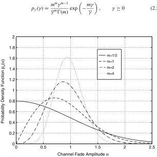
where m is the Nakagami-m fading parameter which ranges from 12 to 1. Figure 2.1 shows the Nakagami-m PDF for D1 and various values of the m parameter. Applying (2.3) shows that the SNR per symbol, , is distributed according to a gamma distribution given by
p⊲⊳D
mmm1 m⊲m⊳exp
m
, ½0 ⊲2.21⊳
0 0.5 1 1.5 2 2.5
0 0.2 0.4 0.6 0.8 1 1.2 1.4 1.6 1.8 2
m=1/2 m=1 m=2 m=4
Channel Fade Amplitude α
Probability Density Function p
α
(
α
)
It can also be shown that the MGF is given in this case by
M⊲s⊳D
1s m
m
⊲2.22⊳
and that the moments are given by [12, Eq. (65)]
E[k]D ⊲mCk⊳ ⊲m⊳mk
k ⊲2.23⊳
which yields an AF of
AFmD 1
m, m½
1
2 ⊲2.24⊳
Hence, the Nakagami-mdistribution spans via themparameter the widest range of AF (from 0 to 2) among all the multipath distributions considered in this book. For instance, it includes the one-sided Gaussian distribution (mD 12) and the Rayleigh distribution (mD1) as special cases. In the limit asm! C1, the Nakagami-m fading channel converges to a nonfading AWGN channel. Furthermore, when m <1, equating (2.14) and (2.24), we obtain a one-to-one mapping between the mparameter and theqparameter, allowing the Nakagami-mdistribution to closely approximate the Nakagami-q(Hoyt) distribution, and this mapping is given by
mD ⊲1Cq 2⊳2
2⊲1C2q4⊳, m1 ⊲2.25⊳ Similarly, whenm >1, equating (2.19) and (2.24) we obtain another one-to-one mapping between the m parameter and the n parameter (or, equivalently, the Rician Kfactor), allowing the Nakagami-m distribution to closely approximate the Nakagami-n(Rice) distribution, and this mapping is given by
mD ⊲1Cn 2⊳2
1C2n2 , n½0 nD
p
m2m
mpm2m, m½1
⊲2.26⊳
Finally, the Nakagami-m distribution often gives the best fit to land-mobile [21–23] and indoor-land-mobile [24] multipath propagation, as well as scintillating ionospheric radio links [9,25–28].
2.2.2 Log-Normal Shadowing
terrain, buildings, and trees. Communication system performance will depend on shadowing only if the radio receiver is able to average out the fast multipath fading or if an efficient microdiversity system is used to eliminate the effects of multipath. Based on empirical measurements, there is a general consensus that shadowing can be modeled by a log-normal distribution for various outdoor and indoor environments [21,29–33], in which case the path SNR per symbol has a PDF given by the standard log-normal expression
p⊲⊳D p
2exp
⊲10 log10⊳ 2 22
⊲2.27⊳
whereD10/ln 10D4.3429, and(dB) and(dB) are the mean and standard deviation of 10 log10, respectively.
The MGF associated with this slow-fading effect is given by
M⊲s⊳' 1 p
Np
nD1
Hxnexp⊲10⊲ p
2xnC⊳/10s⊳ ⊲2.28⊳
where xn are the zeros of the Np-order Hermite polynomial, and Hxn are the weight factors of theNp-order Hermite polynomial and are given by Table 25.10 of Ref. 50. In addition, the moments of (2.27) are given by
E[k]Dexp
k
C
1 2
k
2
2
⊲2.29⊳
yielding an AF of
AFDexp
2 2
1 ⊲2.30⊳
From (2.30) the AF associated with a log-normal PDF can be arbitrarily high. However, as noted by Charash [5, p. 29], in practical situations the standard deviation of shadow fading does not exceed 9 dB [3, p. 88]. Hence, the AF of log-normal shadowing is bounded by 73. This number exceeds the maximal AF exhibited by the various multipath PDFs studied in Section 2.2.1 by several order of magnitudes.
2.2.3 Composite Multipath/Shadowing
vehicles [21,34,35]. This type of composite fading is also observed in land-mobile satellite systems subject to vegetative and/or urban shadowing [36–40]. There are two approaches and various combinations suggested in the literature for obtaining the composite distribution. Here, as an example, we present the composite gamma/log-normal PDF introduced by Ho and St¨uber [35]. This PDF arises in Nakagami-m shadowed environments and is obtained by averaging the gamma distributed signal power (or, equivalently, the SNR per symbol) of (2.21) over the conditional density of the log-normally distributed mean signal power (or equivalently, the average SNR per symbol) of (2.27), giving the following channel PDF:
p⊲⊳D
1
0
mmm1 wm⊲m⊳exp
m
w
p
2wexp
⊲10 log10w⊳ 2 22
dw ⊲2.31⊳
For the special case where the multipath is Rayleigh distributed (mD1), (2.31) reduces to a composite exponential/log-normal PDF which was initially proposed by Hansen and Meno [34].
The MGF is given in this case by
M⊲s⊳' p1
Np
nD1
Hxn⊲110⊲ p
2xnC⊳/10s/m⊳m ⊲2.32⊳
and the moments associated with a gamma/log-no