c
World Scientific Publishing Company 3
ON THE CONVERGENCE OF THE KRIGING-BASED 5
FINITE ELEMENT METHOD
F. T. WONG∗and W. KANOK-NUKULCHAI† 7
School of Engineering and Technology Asian Institute of Technology
9
Pathumthani, 12120, Thailand
Received 13
Accepted
An enhancement of the FEM using Kriging interpolation (K-FEM) was recently pro-15
posed. This method offers advantages over the conventional FEM and mesh-free meth-ods. With Kriging interpolation, the approximated field over an element is influenced 17
not only by its own element nodes but also by a set ofsatellite nodesoutside the ele-ment. This results inincompatibilityalong interelement boundaries. Consequently, the 19
convergence of the solutions is questionable. In this paper, the convergence is investi-gated through some numerical tests. It is found that the solutions of the K-FEM with 21
an appropriate range of parameters converge to the corresponding exact solutions.
Keywords: Finite element; Kriging; convergence. 23
1. Introduction
In the past two decades various mesh-free methods have been developed and applied
25
to solve problems in continuum mechanics [e.g. Liu (2003); Gu (2005)]. These meth-ods have drawn the attention of many researchers partly due to their flexibility
27
in customizing the approximation function for a desired accuracy. Among all the mesh-free methods, those using the Galerkin weak form, such as the element-free
29
Galerkin method (EFGM) [Belytschko (1994)] and the point interpolation methods [Liu (2003)], maintain the same basic formulation as the FEM. However, although
31
the EFGM and its variants have appeared in many academic articles for more than a decade, their applications seem to find little acceptance in real practice. This is
33
in part due to the inconvenience of their implementation, such as the difficulties in constructing mesh-free approximations for highly irregular problem domains and in
35
handling problems of material discontinuity [Liu (2003)].
∗Doctoral candidate.
†Professor of Structural Engineering.
A very convenient implementation of EFGM was recently proposed [Plengkhom
1
and Kanok-Nukulchai (2005)]. Following the work of Gu [2003], Kriging interpo-lation (KI) was used as the trial function. Since KI passes through the nodes and
3
thus possesses the Kronecker delta property, special treatment of boundary con-ditions is not necessary. For evaluating the integrals in the Galerkin weak form,
5
finite elements could conveniently be used as the integration cells. KI was con-structed for each element by the use of a set of nodes in a domain of influence
7
(DOI) composed of several layers of elements. Thus, for 2D problems, the DOI is in the form of a polygon. With this way of implementation, the EGFM of Plengkhom
9
and Kanok-Nukulchai [2005] can be viewed as an FEM with Kriging shape func-tions. This method is referred to as the Kriging-based FEM (K-FEM) in this
11
paper.
The K-FEM retains the advantages of mesh-free methods as follows:
13
(1) Any requirement for high order shape functions can be easily fulfilled without any change to the element structure;
15
(2) The field variables and their derivatives can be obtained with remarkable accu-racy and global smoothness.
17
A distinctive advantage of the K-FEM over other mesh-free methods is that it inherits the computational procedure of the FEM so that existing general purpose
19
FE programs can be easily extended to include this new concept. Thus, the K-FEM has a higher chance to be accepted in practice. The current trend in research
21
on the K-FEM is toward extension and application of this new technique to dif-ferent problems in engineering, such as applications to Reissner–Mindlin (RM)
23
plates [Wong and Kanok-Nukulchai (2006a, b)], problems with material discontinu-ity [Sommanawat and Kanok-Nukulchai (2006)], and adaptive procedure [Mazood
25
and Kanok-Nukulchai (2006)].
Daiet al.[2003] pointed out that the method using the standard Galerkin weak
27
form with KI is nonconforming (incompatible) and so is the K-FEM. The very important issue of incompatibility and its effect on the convergence of the K-FEM
29
have not been addressed in the previous researches. In this paper we address the incompatibility in the K-FEM — the reason why the K-FEM is not conforming is
31
explained and existing techniques for restoring incompatibility are briefly discussed. The convergence is scrutinized through some numerical tests in plane-stress and RM
33
plate problems. First, the weak patch tests for each problem are performed. Then, benchmark problems for plane-stress solids and for RM plates are solved. Relative
35
error norms of displacement and strain energy are utilized to study the convergence. The convergence characteristics of the K-FEM with Gaussian and quartic spline
37
(QS) correlation functions are assessed and compared.
The present paper is organized as follows. Section 2 briefly reviews the
formula-39
tion of KI. Its implementation in plane-stress/plane-strain and RM plate problems is presented in Sec. 3. In Sec. 4, the incompatibility in the K-FEM is discussed.
Numerical studies on the convergence of the K-FEM are presented in Sec. 5, with
1
concluding remarks in Sec. 6.
2. Kriging Interpolation 3
This section presents a review of the KI formulation in the context of the K-FEM. A detailed explanation and derivation of Kriging may be found in the geostatistics
5
literature [e.g. Olea (1999); Wackernagel (1998)].
2.1. Formulation 7
Consider a continuous field variable u(x) defined in a domain Ω. The domain is represented by a set of properly scattered nodesxi,i= 1,2, . . . , N, whereN is the 9
total number of nodes in the whole domain. GivenN field valuesu(x1), . . . , u(xN),
the problem is to obtain an estimated value ofuat a pointx0∈Ω. 11
The Kriging estimated valueuh(x
0) is a linear combination ofu(x1), . . . , u(xn)
in the form
13
uh(x0) = n
i=1
λiu(xi), (1)
whereλi’s are termed (Kriging)weightsandnis the number of nodes surrounding 15
the point x0 inside a subdomain Ωx0 ⊆ Ω. This subdomain is referred to as a
domain of influence (DOI) in this paper. Considering the value of each function
17
u(x1), . . . , u(xn) as the realizations of random variablesU(x1), . . . , U(xn), Eq. (1)
can be written as
19
Uh(x0) = n
i=1
λiU(xi). (2)
The Kriging weights are determined by requiring the estimatorUh(x
0) to be unbi-21
ased, i.e.
E[Uh(x0)−U(x0)] = 0, (3) 23
and byminimizingthe variance of the estimation error,var[Uh(x
0)−U(x0)]. Using
the method of Lagrange for constraint optimization problems, the requirements of minimum variance and unbiased estimator lead to the following Kriging equation system:
Rλ+Pµ=r(x0),
(4)
PTλ=p(x0),
in which
R=
C(h11) · · · C(h1n) · · · ·
C(hn1) · · · C(hnn)
, P=
p1(x1) · · · pm(x1) · · · ·
p1(xn) · · · pm(xn)
λ= [λ1 · · · λn]T, µ= [µ1 · · · µm]T, (6)
r(x0) = [C(h10) C(h20) · · · C(hn0)]T, p(x0) = [p1(x0) . . . pm(x0)]T
(7)
R is an n×n matrix of covariances, C(hij), between two nodal values of U(x) 1
evaluated at{xi,xj}; Pis ann×m matrix of polynomial values at the nodes;λ
is ann×1 vector of Kriging weights;µis anm×1 vector of Lagrange multipliers;
3
r(x0) is an n×1 vector of covariance between the nodes and the node of interest, x0; and p(x0) is anm×1 vector of polynomial basis atx0. In Eqs. (5) and (7), 5
C(hij) =cov[U(xi), U(xj)]. (8)
Solving the Kriging system, Eq. (4), results in Kriging weights, as follows:
7
λT =pT(x0)A+rT(x0)B, (9)
where
9
A= (PTR−1P)−1PTR−1, B=R−1(I−PA). (10) Here,Ais anm×nmatrix,Bis ann×nmatrix, andIis then×nidentity matrix.
11
The expression for the estimated valueuhgiven by Eq. (1) can be rewritten in
matrix form as
13
uh(x
0) =λTd, (11)
in whichd = [u(x1) · · · u(xn)]T is an n×1 vector of nodal values. Since the 15
pointx0is an arbitrary point in the DOI, the symbolx0will henceforth be replaced
by the symbolx. Thus, using the usual finite element terminology, Eq. (11) can be
17
expressed as
uh(x) =N(x)d=
n
i=1
Ni(x)ui, (12) 19
in whichN(x) =λT(x) is the matrix of shape functions.
Two key properties of Kriging shape functions that make them appropriate to be
21
used in the FEM are theKronecker delta(orinterpolation) property andconsistency
property [Gu (2003); Plengkhom and Kanok-Nukulchai (2005)]. Due to the former
23
property, the KI function passes through all nodal values. The consequence of the latter property is that if the basis includes all constants and linear terms, the Kriging
25
shape functions will be able to reproduce a linear polynomial exactly.
2.2. Polynomial basis and correlation function 27
Constructing Kriging shape functions in Eq. (12) requires a polynomial basis func-tion and a model of covariance funcfunc-tion. For the basis funcfunc-tion, besides complete
29
polynomial bases, it is also possible to use incomplete polynomial bases such as bilinear, biquadratic, and bicubic bases for interpolation in a 2D domain (for
comparison, see Noguchi et al. [2000] for polynomial bases in the context of the
1
moving least-squares approximation).
Covariance between a pair of random variables U(x) and U(x +h) can be
3
expressed in terms of the correlation coefficient function or, in short, the corre-lation function, as follows:
5
ρ(h) =C(h)
σ2 , (13)
whereρ(h) is the correlation function,σ2=var[U(x)], andhis a vector separating 7
two points,xandx+h. According to Gu [2003],σ2has no effect on the final results
and so in this study it is taken as 1. One of the widely used correlation models in
9
the area of computational mechanics is the Gaussian correlation function [e.g. Gu (2003); Daiet al.(2003); Wong and Kanok-Nukulchai (2006a)], viz.
11
ρ(h) =ρ(h) = exp
− θh d
2
, (14)
where θ > 0 is the correlation parameter, h = h, i.e. the Euclidean distance
13
between the pointsxandx+h, anddis a scale factor for normalizing the distance. In this study, d is taken to be the maximum distance between any pair of nodes
15
in the DOI. Besides the Gaussian, we recently introduced the quartic spline (QS) correlation function [Wong and Kanok-Nukulchai (2006a,b)] as follows:
17
ρ(h) =
1−6 θh d
2
+ 8 θh d
3
−3 θh d
4
for 0≤θh d ≤1,
0 forθh
d >1.
(15)
Our study shows that using the QS correlation function, Kriging shape functions
19
are not sensitive to the change in the parameterθ.
The proper choice of the parameter θ is very important, because it affects the
21
quality of KI. In order to obtain reasonable results in the K-FEM, Plengkhom and Kanok-Nukulchai [2005] suggested a rule of thumb for choosingθ; namely,θshould
23
be selected so that it satisfies the lower bound,
n i=1
Ni−1
≤1×10⁻¹⁰+a, (16)
25
whereais the order of the basis function, and also satisfies the upper bound,
det(R)≤1×10−b, (17)
27
where b is the dimension of the problem. For a 2D problem with a cubic basis function, for example,a= 3 andb= 2.
29
Numerical investigations on the upper and lower bound values ofθ[Wong and Kanok-Nukulchai (2006a)] revealed that the parameter bounds vary with respect
31
lower and upper bound values ofθ satisfying Eqs. (16) and (17), we proposed the
1
following explicit parameter functions for practical implementation of the K-FEM for problems with 2D domains.
3
For the Gaussian correlation parameter, the parameter function is
θ= (1−f)θlow+f θup, 0≤f ≤0.8, (18)
5
wherefis a scale factor, andθlow, andθup, are the lower and upper bound functions:
θlow=
0.08286n−0.2386 for 3≤n <10,
−8.364E−4n2+ 0.1204n−0.5283 for 10≤n≤55,
0.02840n+ 2.002 forn >55,
(19)
θup=
0.34n−0.7 for 3≤n <10,
−2.484E−3n2+ 0.3275n−0.2771 for 10≤n≤55,
0.05426n+ 7.237 forn >55.
(20)
For the QS correlation parameter, the parameter function is
θ=
0.1329n−0.3290 for 3≤n <10,
1 forn≥10. (21)
7
2.3. Layered-element domain of influence
Let us consider a 2D domain mesh using triangular elements, as illustrated in Fig. 1.
9
For each element, KI is constructed based upon a set of nodes in a polygonal DOI encompassing a predetermined number of layers of elements. The KI function over
11
the element is given by Eq. (12). By combining the KI of all elements in the domain, the global field variable is approximated by piecewise KI. This way of approximation
13
is very similar to the approximation in the conventional FEM.
It should be mentioned here that it is also possible to use quadrilateral elements
15
to implement the concept of a layered-element DOI. Mesh with triangular elements
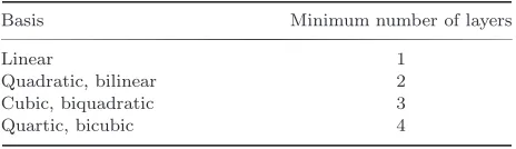
Table 1. Minimum number of layers for various basis functions.
Basis Minimum number of layers
Linear 1
Quadratic, bilinear 2
Cubic, biquadratic 3
Quartic, bicubic 4
is chosen in this study, owing to its flexibility in representing complex geometry and
1
its ease in being automatically generated.
The number of layers for each element must cover a number of nodes in such a
3
way that the Kriging equation system, Eq. (4), is solvable. If anm-order polynomial basis is employed, the DOI is required to cover a number of nodes,n, that is equal to
5
or greater than the number of terms in the basis function, i.e.n≥m. Based on our experience, the minimum number of layers for different polynomial bases is listed in
7
Table 1. As the number of layers increases, the computational cost becomes higher. Thus we recommend the use of a minimum number of layers for each polynomial
9
basis.
3. Formulation 11
3.1. K-FEM for plane-strain/plane-stress solids
The governing equations for plane-strain/plane-stress problems in the Cartesian
13
coordinate system can be written in a weak form, as follows:
V
δεTσdV =
V
δuTbdV +
S
δuTtdS, (22)
15
whereu={u v}T is the displacement vector,ε={ε
x εy γxy}T is the vector of
2D strain components,σ={σx σy τxy}T is the vector of 2D stress components, 17
b={bx by}T is the body force vector;t={tx ty}T is the surface traction force
vector, V is the 3D domain occupied by the solid body, andS is the surface on
19
which the tractiontis applied.
Suppose that the domain V is subdivided by a mesh of Nel elements and N 21
nodes. To obtain an approximate solution using the concept of KI with a layered-element DOI, for each layered-elemente= 1,2, . . . , Nelthe displacement componentsuand 23
v are approximated by KI as follows:
u(x, y)≃ n
i=1
Ni(x, y)ui, v(x, y)≃ n
i=1
Ni(x, y)vi (23) 25
Here,Ni(x,y) denotes the Kriging shape function associated with node i; ui and
vi are nodal displacement components in the xandy directions, respectively; and 27
n is the number of nodes in the DOI of an element, which generally varies from element to element. Employing the standard formulation procedure of the FEM
[e.g. Cooket al. (2002); Zienkiewicz and Taylor (2000)], we may obtain the
equilib-1
rium equation for each element as follows:
kede=fe, (24)
3
where the element stiffness matrix (2n×2n)
ke=
Ve
BeTEBedV , (25)
5
the displacement vector (2n×1)
de={u1 v1 u2 v2 · · · un vn}T, (26) 7
and the consistent nodal force vector of elemente(2n×1)
fe=
Ve
NeTbedV +
Se
NeTtedS. (27)
9
MatrixNeis the Kriging shape function matrix, i.e.
Ne=
N1 0 N2 0 · · · Nn 0
0 N1 0 N2 · · · 0 Nn
, (28)
11
Beis the element strain-displacement matrix, i.e.
Be=
N1,x 0 N2,x 0 · · · Nn,x 0
0 N1,y 0 N2,y · · · 0 Nn,y
N1,y N1,x N2,y N2,x · · · Nn,y Nn,x
, (29)
13
andE is the constitutive matrix, which, for the case of isotropic material, can be expressed in terms of modulus elasticityE and Poisson’s ratioν as follows:
15
E= E¯ 1−ν¯2
1 ¯ν 0
¯
ν 1 0 0 0 (1−ν¯)/2
, (30)
with 17 ¯ E= E E
1−ν2
, ν¯=
ν for plane stress, ν
1−ν for plane strain.
(31)
Veis the 3D domain of element eandSe is the surface of elemente on which the 19
tractiontis applied.
For a triangular element of thicknesshand areaAe, with traction force on edge
se, Eqs. (25) and (27) can be expanded as follows:
ke=h
Ae
BeTEBe, (32)
fe=h
Ae
NeTbedA+, h
se
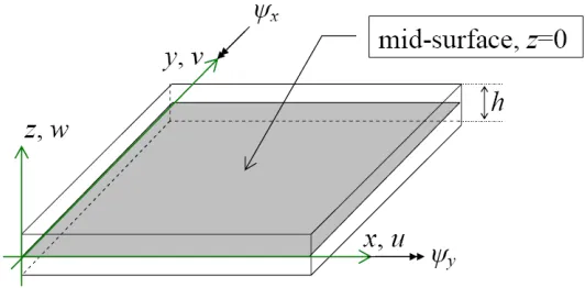
Fig. 2. Positive directions for displacement and rotation components.
3.2. K-FEM for Reissner–Mindlin plates 1
Consider a plate of uniform thickness, h, homogeneous, referred to a three-dimensional Cartesian coordinate system with the x–y plane lying on the middle
3
surface of the plate (Fig. 2). Its domain,V, is defined as
V =
(x, y, z)∈R3|z∈
−h 2, h 2
,(x, y)∈S⊂R2
. (34)
5
Rotation of a normal line has two components, namelyψxandψy. The positive sign
convention for these rotation components and displacement components is shown in
7
Fig. 2. For small displacement and rotation, the displacement field is described by
u3D=
u v w =
−zψx(x, y) −zψy(x, y)
w(x, y)
, (35) 9
wherew(x, y) is the deflection of a point initially lying on the reference plane,S, and
ψx(x, y) andψy(x, y) are the normal line rotation components around its midpoint 11
with respect to the –yandxdirections, respectively.
The governing equations for static deflection of RM plates under transversal
13
loadq(x, y) can be written in a weak form as follows:
S
δκTDbκdS+
S
δεTsDsεsdS=
S
δuTpdS. (36)
15
In this equation,
κ={ψx,x ψy,y ψx,y+ψy,x}T (37) 17
is the curvature vector,
εs={γx z γy z}T (38)
19
is the transverse shear vector,
u={w ψx ψy}T (39)
is the vector of three independent field variables for RM plates,
1
p={q 0 0}T (40)
is the surface force vector,
3
Db =
Eh3
12(1−ν2)
1 ν 0
ν 1 0 0 0 (1−ν)/2
(41)
is the elasticity matrix for bending deformation, and
5
Ds=Gkh
1 0 0 1
(42)
is the elasticity matrix for transverse shear deformation. Here,
7
G= E
2(1 +ν) (43)
is the shear modulus andkis a shear correction factor to account for the parabolic
9
zdirection variation of transverse shear stress. The accepted value ofkfor a homo-geneous plate isk= 5/6 [Cooket al.(2002)].
11
Suppose that the domainS is subdivided by a mesh ofNel triangular elements
and N nodes. To obtain an approximate solution using the concept of KI with a layered-element DOI, for each elemente= 1,2, . . . , Nel the plate field variables are
approximated by KI as follows:
w(x, y)≃ n
i=1
Ni(x, y)wi,
ψx(x, y)≃ n
i=1
ηi(x, y)ψxi, ψy(x, y)≃ n
i=1
ξi(x, y)ψyi. (44)
HereNi(x, y),ηi(x, y) andξi(x, y) denote Kriging shape functions associated with
nodeifor approximating defection and rotation in they direction, and rotation in
13
thex-direction, respectively; and wi,ψxi, andψyi are nodal deflection, and nodal
rotation in the –y direction, and nodal rotation in the x direction, respectively.
15
Shape functionsNi,ηi, andξi do not have to be the same; they are independent of
each other. In this study, however, they are taken to be the same, i.e.
17
ηi(x, y) =ξi(x, y) =Ni(x, y). (45)
Inserting Eq. (44) into the variational equation of RM plates, Eq. (36), leads to the
19
following discretized equilibrium equation for each element:
kede=fe, (46)
in which the element stiffness matrix (3n×3n) is
1
ke=keb+kes=
Se
BeTb DbBebdS+
Se
BeTs DsBesdS, (47)
the element nodal displacement vector (3n×1) is
3
de={w1 ψx1 ψy1 w2 ψx2 ψy2 · · · wn ψx n ψyn}T, (48)
and the element nodal force vector (3n×1) is
5
fe=
Se
NeTpedS. (49)
In Eqs. (47) and (49), matricesNe,Beb, andBesare defined as follows:
Ne=
N1 0 0 · · · Nn 0 0
0 N1 0 · · · 0 Nn 0
0 0 N1 · · · 0 0 Nn
, (50)
Beb =
0 N1,x 0 · · · 0 Nn,x 0
0 0 N1,y · · · 0 0 Nn,y
0 N1,y N1,x · · · 0 Nn,y Nn,x
, (51)
Bes=
N1,x −N1 0 · · · Nn,x −Nn 0
N1,y 0 −N1 · · · Nn,y 0 −Nn
. (52)
3.3. Global discretized equilibrium equation 7
The global discretized equilibrium equation,
KD=F, (53)
9
can be obtained from the element equilibrium equations — Eq. (24) for plane-stress/plane-strain problems and Eq. (46) for RM plates — by using the assembly
11
procedure, i.e.
K=ANel
e=1k
e, D=ANel
e=1d
e, F=ANel
e=1f
e. (54) 13
HereKis the global stiffness matrix,Dis the global nodal displacement vector,F
is the global nodal force vector, and ANel
e=1 denotes the assembly operator. It should 15
be mentioned here that the assembly process for each element involvesall nodes in the element’s DOI, and not only the nodes within the element as in the conventional
17
FEM.
4. Incompatibility in the K-FEM 19
As described in Sec. 2, the KI is constructed for each element using a set of nodes, within and outside the element, in a predetermined layered-element DOI.
21
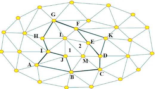
Fig. 3. The domain of influence of element 1 and element 2.
However, along the element edges between two adjacent elements the function is
1
not perfectly continuous, because the KI for each of the two neighboring elements is constructed using a different set of nodes.
3
For illustration, we consider element 1 and element 2 in a 2D domain as shown in Fig. 3 and suppose that we use two element layers as the DOI for each element.
5
Polygon A-B-C-D-E-F-G-H-I is the DOI for element 1 and polygon B-C-D-K-F-G-H-I-J is the DOI for element 2. The KI within element 1 is constructed using the
7
12 nodes in the first polygon, while the KI within element 2 is constructed using the 11 nodes in the second polygon. As a result, the function along the edge LM of
9
element 1 is different from the function along the edge LM of element 2. In other words, the displacement function is not continuous across the common edge LM of
11
the two neighboring elements. The foregoing explanation is principally the same as that presented by Daiet al.[2003] in the context of the EFGM with KI.
13
To illustrate further the interelement incompatibility in the K-FEM, we consider again the domain shown in Fig. 3 and suppose now that the value at node K is 1
15
and the other nodal values are 0. According to the KI of element 1, the function along the interface LM is a zero function since the value at node K does not have
17
any effect on the KI within element 1. On the contrary, according to element 2, the function along LM is not a zero function because the shape function associated
19
with node K is not 0 between nodes L and M.
Thus it is apparent that the K-FEM does not satisfy the interelement
compati-21
bility requirement (nonconforming), except for the K-FEM with a linear basis and one layer DOI. Is this incompatibility acceptable? It is acceptable if it tends to zero
23
as the mesh is repeatedly refined [Cooket al.(2002)]. In other words, the interele-ment compatibility needs only to be satisfied in the limit as the size of the eleinterele-ment
25
tends to zero. This is assessed through the weak patch test and convergence studies in the following section.
It should be mentioned here that it is also possible to employ a constrained
1
variational equation in the K-FEM to deal with the incompatibility [e.g. Daiet al.
(2003)]. This approach, however, will destroy the key advantage of the K-FEM
3
mentioned in Sec. 1, namely its ease of implementation in a general purpose finite element program. It is for this reason that we do not resort to this approach to deal
5
with the incompatibility.
After completion of the present study, we became aware of recent works by
7
G. R. Liu’s group on a class of computational methods based on the Galerkin for-mulation using the so-called generalized gradient smoothing technique [Liu (2008)].
9
Examples of the methods in this class are the node-based smoothed point polation method (NS-PIM, originally called the linearly conforming point
inter-11
polation method) [Liu et al. (2005); Zhang et al. (2007)] and the node-based smoothed radial point interpolation method (NS-RPIM) [Liuet al.(2006); Liet al. 13
(2007)]. In these methods, the compatibility of the incompatible node-based inter-polations was restored by using the stabilized conforming nodal integration
pro-15
posed by Chenet al.[2001]. Nevertheless, the methods entail creation of smoothing domains that are generally different from the original finite element mesh. A
tech-17
nique for constructing smoothing domains should be judiciously selected or invented in order to preserve the simplicity of the K-FEM. It seems that the edge-based
19
smoothing technique [Liu (2008) and references therein], in which the smoothing domains are created based on edges of the elements, is a good choice for
imple-21
mentation of the gradient smoothing technique in the K-FEM. This needs further research.
23
5. Numerical Tests
In the following tests, the integrals over each triangular element in the expressions
25
for element stiffness matrices, Eqs. (32) and (47), and for nodal force vectors, Eqs. (33) and (49), were computed using the six-point quadrature rule for triangles [e.g.
27
Hughes (1987)]. This rule was selected because it may give results that are reason-ably accurate yet inexpensive in terms of computational cost. For computing the
29
line integral in Eq. (33), the two-point Gaussian quadrature for line integrals was used, since it can yield an exact nodal force vector for edge traction force with cubic
31
distribution or less.
Abbreviations in the form of P*-*-G* or P*-*-QS, in which the asterisk denotes
33
a number, are adopted in this section to designate various options of the K-FEM. The first syllable denotes a polynomial basis with the order indicated by the number
35
next to letter P. The middle asterisk denotes the number of layers. The last syllable denotes the Gaussian correlation function with the adaptive parameter given by
37
Eq. (18) and with the scale factor f indicated by the number next to the letter G (in percent); QS denotes the quartic spline correlation function with the
adap-39
element layers, Gaussian correlation function with midvalue parameter function,
1
i.e.f = 0.5.
5.1. Plane-stress/plane-strain solids 3
To study the convergence of the K-FEM for plane-stress/plane-strain solids, two measures of error were utilized. The fist one is a relative L2 error norm of 5
displacement, defined as
ru= V
(uapp−uexact)T(uapp−uexact)dV
V(uexact)TuexactdV
1/2
, (55)
7
whereuappanduexactare approximate and exact displacement vectors, respectively.
The second one is a relative error norm of strain energy, defined as
9
rε= V
(εapp−εexact)TE(εapp−εexact)dV
V (εexact)TEεexactdV
1/2
, (56)
where εapp andεexact are approximate and exact strain vectors, respectively. For 11
computing these relative errors, the 13-point quadrature rule for triangles was employed for each element.
13
5.1.1. Weak patch test
We patch test is a test on a “patch” of finite elements with states of constant strains
15
or constant stresses. Since the K-FEM is nonconforming, it will not pass the patch test for a patch with a large size of elements. Passing the patch test for a large size of
17
elements, however, is not a necessary condition for convergence. Thenecessaryand
sufficientcondition for convergence is to pass the patch test in the limit, as the size
19
of the elements in the patch tends to zero [Zienkiewicz and Taylor (2000); Razzaque (1986)], provided that the system of equations is solvable and all integrations are
21
exact. This kind of test is referred to asa weak patch test[Zienkiewicz and Taylor (2000); Cooket al. (2002)].
23
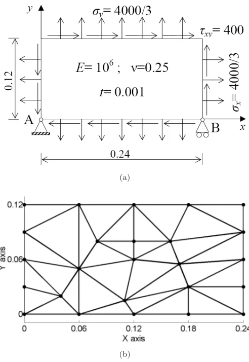
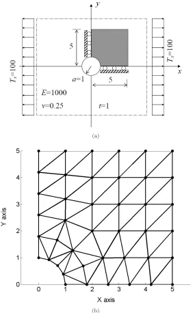
The patch used for the weak patch test is shown in Fig. 4(a). It was adapted from the patch proposed by MacNeal and Harder [1985]. In order to be consistent with
25
the displacement fieldu= 10−3(x+y/2),v= 10−3(y+x/2),u= 0.24×10⁻³, and
v= 0.12×10⁻³were prescribed at node B. The initial course mesh, which includes
27
25 nodes, is shown in Fig. 4(b). We defined the element characteristic size for this meshhc= 0.06. Subsequently, mesh refinements were performed by subdividing the 29
elements.
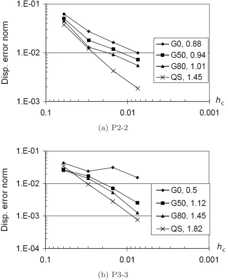
The following K-FEM options were used for the weak patch test: P2-2 with
31
G0, G50, G80, QS and P3-3 with G0, G50, G80, QS. Displacement error norms of the K-FEM solutions are plotted against element characteristic sizes in Fig. 5. The
33
average convergence rate (R) of each option is also shown in the legend. The figure indicates that the K-FEM does not pass the test in any mesh but the solutions
(a)
(b)
Fig. 4. (a) A patch under constant stresses and (b) its initial mesh for the weak patch test.
converge. For the K-FEM of option P3-3-G0, however, the convergence is doubtful.
1
Therefore, we conclude that the K-FEMpasses the weak patch test, except for that with option P3-3-G0. For the K-FEM with Gaussian correlation functions, as the
3
parameter θ comes closer to the upper bound values, the convergence rate and accuracy increase. The K-FEM with the QS is the best in terms of the convergence
5
rate (R= 1.45 for P2-2 andR= 1.82 for P3-3).
The strain energy error norms vs. element characteristic sizes are shown in Fig. 6.
7
These energy errors are mainly due to “gaps” or “overlaps” along the interface between two elements, because the roundoff and numerical integration errors are
9
negligible. Therefore, in this case the energy error may serve as a measure of the degree of incompatibility of the K-FEM. The figure shows that the incompatibilities
11
(a) P2-2
(b) P3-3
Fig. 5. Relative error norm of displacement vs. element characteristic size for the patch analyzed using the K-FEM with: (a) P2-2, (b) P3-3. The number after the code for the K-FEM option in the legend indicates the average convergence rate.
K-FEM with the QS correlation function is “more compatible” than that with the
1
Gaussian.
5.1.2. An infinite plane-stress plate with a hole 3
An infinite plane-stress plate with a circular hole of radius a = 1 was subjected to a uniform tensionTx = 100 at infinity [Tongsuk and Kanok-Nukulchai (2004)] 5
[Fig. 7(a)]. In view of the symmetry, only the upper right quadrant of the plate, 0≤
x≤5 and 0≤y≤5, was analyzed. Zero normal displacements were prescribed on
7
the symmetric boundaries and the exact traction boundary conditions were imposed on the right (x= 5) and top (y= 5) edges.
9
The initial course mesh of 42 nodes is shown in Fig. 7(b). The element charac-teristic size for this problem is taken as the distance between two nodes at the right
11
or top edge, i.e. hc = 1. Subsequently, the mesh was refined by subdividing the
previous element into four smaller elements. The refined meshes considered in this
13
test are meshes withhc= 0.5 (141 nodes) andhc= 0.25 (513 nodes). In performing
(a) P2-2
(b) P3-3
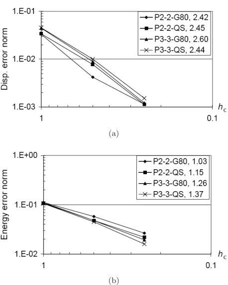
Fig. 6. Relative error norms of strain energy vs. element characteristic sizes for the patch analyzed using the K-FEM with: (a) P2-2, (b) P3-3.
f = 0.79 was used in place off = 0.8, because the use off = 0.8 resulted in det(R)
1
exceeding the upper bound criterion, Eq. (17), for some elements.
The convergence characteristics for displacement and strain energy are shown in
3
Figs. 8(a) and 8(b), respectively. The figures indicate that the rates of convergence of all K-FEM options are nearly equal, for displacement as well as strain energy.
5
The fastest convergence rate in terms of the displacement error is achieved by the K-FEM with P3-3-G80 (the rateR= 2.60), while the fastest one in terms of the strain
7
energy error is the K-FEM with P3-3-QS (R = 1.37). Theoretically, the accuracy and convergence rate of the K-FEM with a cubic basis higher than those with a
9
quadratic basis. However, this is not the case because of the incompatibilities of the K-FEM.
11
5.2. Reissner–Mindlin plates
The convergence of the K-FEM for RM plates was assessed in terms of the relative
13
L2 error norm of displacement, viz.
ru=
uapp3D −uexact
3D
uexact
3D
, (57)
(a)
(b)
Fig. 7. (a) An infinite plate with a circular hole and (b) the initial mesh of the shaded area.
where uapp3D and uexact
3D are approximate and exact displacement vectors of the 3D 1
solid, respectively. The displacement norm in Eq. (57) was expanded as follows:
u3D= V
uT3Du3DdV
1/2
=
V
(u2+v2+w2)dV
1/2
. (58)
(a)
(b)
Fig. 8. Relative error norms of (a) displacement and of (b) strain energy and their convergence rates for the holed plate.
Substituting theu,v, andwin this equation with those stated in Eq. (35) and then
1
integrating over the thickness resulted in
u3D= h
S
w2dS+h3
3
S
(ψ2
x+ψy2)dS
1/2
. (59)
3
As in the previous tests, the 13-point quadrature rule for triangles was employed to evaluate the integrals in this equation for each element.
5
5.2.1. Weak patch tests
The same patch and meshes as in the previous patch test (Fig. 4) were used in the
7
following tests, except for the loading condition and the thickness. Two conditions of the patch were considered: constant curvature and constant transverse shear
9
strain. The length-to-thickness ratio of the patch was differently specified for each condition of the tests. Based on the study of the performance of various K-FEM
11
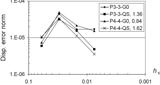
options in alleviating shear locking [Wong and Kanok-Nukulchai (2006a, b)], the following K-FEM options were used for the patch tests: P3-3-G0, P3-3-QS, P4-4-G0,
13
5.2.1.1. Constant curvature condition
1
The boundary of the patch was imposed by the essential boundary conditions as presented by MacNeal and Harder [1985], i.e.
w=10−
3(x2+xy+y2)
2 , (60)
ψx=
∂w ∂x = 10−
3x+y
2
, ψy=
∂w ∂y = 10−
3x
2 +y
. (61)
These fields lead to the following constant curvatures and moments:
κ={1 1 1}T ×10−3, M=−
10
9 10
9 1 3
T
×10−7. (62)
3
Shear strains and shear stresses corresponding to these constant curvatures are zero. The length-to-thickness ratio of the patch was set to 240 (h = 0.001) in order to
5
represent thin plates.
Displacement error norms of the K-FEM solutions are plotted against element
7
characteristic sizes in Fig. 9. It can be seen that from the second mesh (hc= 0.03)
until the last mesh (hc = 0.0075) the solutions of the K-FEM converge, except 9
for the K-FEM with option P3-3-G0. The solutions for the mesh of hc = 0.06
(25 nodes) are exceptionally accurate, because 16 of the 25 nodes are located at
11
the boundary and accordingly imposed by the boundary conditions (60). Thus, the nodal displacements associated with the 16 boundary nodes are automatically
13
exact. In addition, for a cases of a relatively small number of nodes in a domain, the K-FEM may yield extraordinarily accurate results because the KI is close to
15
a polynomial function of higher order than the basis function. We conclude that the K-FEM with options P3-3-QS, P4-4-G0, and P4-4-QSpassthe weak constant
17
curvature patch test but the K-FEM with P3-3-G0does notpass. The K-FEM with
Fig. 9. Relative error norm of displacement vs. element characteristic size for the constant curvature patch test. The numbers in the legend indicate the average convergence ratesfrom the second mesh
the QS correlation function has a better convergence characteristic than that with
1
G0. This finding is similar to the one regarding the plane-stress condition.
Constant transverse shear-strain condition 3
A state of constant transverse shear strains and zero curvatures, i.e.
εs={1 1}T×10−6, κ={0 0 0}T, (63) 5
can be obtained, with all equilibrium equations satisfied, only for the extreme case of thick plates [Batoz and Katili (1992)]. In this test, an extremely thick plate with
7
the length-to-thickness ratio 0.0024 (h = 100) was considered. The displacement fields leading to the constant shear strains, Eq. (62), are as follows:
9
w= 10−6x+y
2 , ψx=− 1 2 ×10
−6, ψ
y=−1
2 ×10
−6. (64)
The shear forces corresponding to the constant shear strains are
11
Q=
100 3
100 3
T
. (65)
The test was performed by imposing nodal values on the boundary according to
13
the fields stated by Eq. (63). The error indicator used in this test is the relativeL2
error norm of deflection, defined as
15
rw=
S(w
app−wexact)2dS
S(wexact)2dS
1/2
. (66)
This indicator was used here instead of the displacement error norm, Eq. (57),
17
because the thickness of the plate was extremely large so that if we used Eq. (57), the norm would be dominated by the rotation errors. We found that these rotation
19
errors are relatively constant for different degrees of mesh refinements.
The plot of the relative deflection error norms for the K-FEM with different
1
analysis options is shown in Fig. 10. It can be seen that all of the options lead to converging solutions and therefore theypassthe weak constant shear patch test. As
3
in the previous test, the accuracy and convergence rate of the K-FEM with QS are better than those with G0.
5
5.2.2. A thin square plate
We considered a hard simply supported square plate of lengthL= 100 and
length-7
to-thickness ratio L/h = 100 under uniform transverse loadq = −1×10⁻⁶. The modulus of elasticity is E = 2×10⁶ and Poisson’s ratio is v = 0.3. To study 9
the convergence of the K-FEM solutions, a quadrant of the plate was discretized with different degrees of mesh refinement: 4×4 (hc = 12.5, Fig. 11), 6×6 (hc = 11
8.33), . . . ,12×12 (hc = 4.17). The meshes were automatically generated using
the Delaunay algorithm and thus the triangles had random orientation, such as
13
shown in Fig. 11. The K-FEMs with P3-3-QS and P4-4-QS were chosen in this and subsequent tests because they showed good performance both in the shear locking
15
study [Wong and Kanok-Nukulchai (2006a, b)] and in patch tests. In computing the displacement error norms, Eq. (57), the exact displacement fields according to
17
the thick plate theory [Reissman (1988)] were used.
The displacement error norms are plotted against element characteristic sizes
19
in Fig. 12. The figure shows excellent convergence characteristics. The results with
Fig. 12. Relative error norms of displacement and their convergence rates for the square plate.
option P4-4-QS, as expected, are more accurate than those with P3-3-QS. However,
1
the best converge rate is achieved for P3-3-QS withR= 5.54. The reason for this is that the incompatibilities in the K-FEM with P3-3-QS diminished faster than that
3
in the K-FEM with P4-4-QS.
5.2.3. A thick circular plate 5
A clamped circular plate of diameterD= 100 and length-to-thickness ratioD/h= 5 was considered. The uniform load intensity and material properties were the
7
same as in the previous test (the thin square plate). A quadrant of the plate was discretized with different degrees of mesh refinement, as shown in Fig. 13. The
9
element characteristic sizehc was defined as the length of the first line segment on
thex axis (which is one of the edges of the triangle in the center). In computing
11
the displacement error norms, the exact solutions based on the thick plate theory [Reismann (1988)] were used.
13
The convergence of the solutions in terms of the displacement error norm is shown in Fig. 14. The figure indicates that the average convergence rates for
P3-15
3-QS and P4-4-QS are nearly equal. The solutions of P3-3-QS are slightly more accurate that those of P4-4-QS. This fact disagrees with the usual tendency in the
17
standard FEM, namely the higher the degree of shape functions, the more accurate the results. This disagreement occurs because in this problem the incompatibility
19
in the K-FEM with P4-4-QS is more severe than that in the K-FEM with P3-3-QS.
6. Conclusions 21
The convergence characteristics of the K-FEM with different options have been studied in the context of plane stress and Reissner–Mindlin plate problems through
23
some numerical tests. It was found that the K-FEM with different options passed the weak patch tests except for the K-FEM with P3-3-G0. For the K-FEM with the
25
Gaussian correlation function, the convergence characteristics were better as the correlation parameters were closer to the upper bound. The K-FEM with the QS
(a) Mesh No. 1: 34 nodes, 47 elements,hc= 10
(b) Mesh No. 2: 43 nodes, 62 elements,hc= 8
(c) Mesh No. 3: 76 nodes, 119 elements,hc= 5
(d) Mesh No. 4: 208 nodes, 359 elements,hc= 2.2
Fig. 14. Relative error norms of displacement and their convergence rates for the circular plate.
correlation function had better convergence characteristics than that with the
Gaus-1
sian as its solutions were not sensitive to the change of the correlation parameter. The numerical tests with several benchmark problems demonstrated good and
reli-3
able convergence characteristics of the K-FEM using QS correlation functions. Passing the weak patch tests indicates that the incompatibility decreases as the
5
mesh is refined. Therefore, the convergence of the K-FEM with appropriate options is guaranteed. The use of the QS correlation function in a K-FEM for analyses of
7
two-dimensional problems is thus recommended. The results of the present study confirm that the K-FEM is a viable alternative to the conventional FEM and has
9
great potential in engineering applications. Future research may be directed at implementation of the generalized gradient smoothing technique [Liu (2008)] in
11
the K-FEM.
References 13
Batoz, J. L. and Katili, I. [1992] On a simple triangular Reissner/Mindlin plate element based on incompatible modes and discrete constraints,Int. J. Numer. Meth. Eng.35,
15
1603–1632.
Belytschko, T., Lu, Y. Y. and Gu, L. [1994] Element-free Galerkin methods,Int. J. Numer.
17
Meth. Eng.37, 229–256.
Chen, J. S., Wu, C. T., Yoon, S. and You, Y. [2001] A stabilized conforming nodal inte-19
gration for Galerkin mesh-free methods,Int. J. Numer. Meth. Eng.50, 435–466.
Cook, R. D., Malkus, D. S., Plesha, M. E. and Witt, R. J. [2002]Concepts and Applications
21
of Finite Element Analysis, 4th edn. (John Wiley and Sons, Madison).
Dai, K. Y., Liu, G. R., Lim, K. M. and Gu, Y. T. [2003] Comparison between the radial 23
point interpolation and the Kriging interpolation used in meshfree methods,Comput. Mech.32, 60–70.
25
Gu, L. [2003] Moving Kriging interpolation and element-free Galerkin method, Int. J. Numer. Meth. Eng.56, 1–11.
27
Gu, Y. T. [2005] Meshfree methods and their comparisons,Int. J. Comput. Meth.2, 477–
515. 29
Hughes, T. J. R. [1987] The Finite Element Method: Linear Static and Dynamic Finite Element Analysis(Prentice-Hall, New Jersey).
Kokaew, N. [2003] Triangular plate bending element based on moving least squares shape 1
functions. Master of Engineering thesis, Asian Institute of Technology, Pathumthani. Li, Y., Liu, G. R., Luan, M. T., Dai, K. Y., Zhong, Z. H., Li, G. Y. and Han, X. [2007] 3
Contact analysis for solids based on linearly conforming radial point interpolation method,Comput. Mech.39, 537–554.
5
Liu, G. R. [2003]Mesh Free Methods(CRC, Boca Raton).
Liu, G. R. [2008] A generalized gradient smoothing technique and the smoothed bilin-7
ear form for Galerkin formulation of a wide class of computational methods, Int. J. Comput. Meth.5, 199–236.
9
Liu, G. R., Li, Y., Dai, K. Y., Luan, M. T. and Xue, W. [2006] A linearly conforming radial point interpolation method for solid mechanics problems,Int. J. Comput. Meth.
11
3, 401–428.
Liu, G. R., Zhang, G. Y., Dai, K. Y., Wang, Y. Y., Zhong, Z. H., Li, G. Y. and Han, 13
X. [2005] A linearly conforming point interpolation method (LC-PIM) for 2D solid mechanics problems,Int. J. Comput. Meth.2, 645–665.
15
MacNeal, R. H. and Harder, R. L. [1985] A proposed standard set of problems to test finite element accuracy,Finite Elements in Analysis and Design1, 3–20.
17
Mazood, Z. and Kanok-Nukulchai, W. [2006] An adaptive mesh generation for Kriging element-free Galerkin method based on Delaunay triangulation, inEmerging Trends:
19
Keynote Lectures and Symposia — Proc. 10th East-Asia Pacific Conf. Struct. Eng. Const.(3–5 Aug. 2006, Bangkok), pp. 499–508.
21
Noguchi, H., Kawashima, T. and Miyamura, T. [2000] Element free analyses of shell and spatial structures,Int. J. Numer. Meth. Eng.47, 1215–1240.
23
Olea, R. A. [1999]Geostatistics for Engineers and Earth Scientists(Kluwer, Boston). Plengkhom, K. and Kanok-Nukulchai, W. [2005] An enhancement of finite element meth-25
ods with moving Kriging shape functions,Int. J. Comput. Meth.2, 451–475.
Razzaque, A. [1986] The patch test for elements,Int. J. Numer. Meth. Eng.22, 63–71.
27
Reissmann, H. [1988] Elastic Plates: Theory and Application (John Wiley and Sons, New York).
29
Sommanawat, W. and Kanok-Nukulchai, W. [2006] The enrichment of material discontinu-ity in moving Kriging methods, inEmerging Trends: Keynote Lectures and Symposia —
31
Proc. 10th East-Asia Pacific Conf. Struct. Eng. Const. (3–5 Aug. 2006, Bangkok), pp. 525–530.
33
Tongsuk, P. and Kanok-Nukulchai, W. [2004] Further investigation of element-free Galerkin method using moving Kriging interpolation,Int. J. Comput. Meth. 1, 345–
35
365.
Wackernagel, H. [1998]Multivariate Geostatistics, 2nd edn. (Springer, Berlin). 37
Wong, F. T. and Kanok-Nukulchai, W. [2006a] Kriging-based finite element method for analyses of Reissner-Mindlin plates, inEmerging Trends: Keynote Lectures and
Sym-39
posia — Proc. 10th East-Asia Pacific Conf. Struct. Eng. Const. (3–5 Aug. 2006, Bangkok), pp. 509–514.
41
Wong, F. T. and Kanok-Nukulchai, W. [2006b] On alleviation of shear locking in the Kriging-based finite element method, inProc. Int. Civil Eng. Conf. “Towards
Sustain-43
able Engineering Practice”(25–26 Aug. 2006, Surabaya), pp. 39–47.
Zhang, G. Y., Liu, G. R., Wang, Y. Y., Huang, H. T., Zhong, Z. H., Li, G. Y. and 45
Han, X. [2007] A linearly conforming point interpolation method (LC-PIM) for three-dimensional elasticity problems,Int. J. Numer. Meth. Eng.72, 1524–1543.
47
Zienkiewicz, O. C. and Taylor, R. L. [2000]The Finite Element Method. Vol. 1: The Basis, 5th edn. (Butterworth Heinemann, Oxford).
![Fig. 1. Domain of influence for element el with one, two, and three layers of elements [Plengkhomand Kanok-Nukulchai (2005)].](https://thumb-ap.123doks.com/thumbv2/123dok/1552326.2047733/6.595.176.413.556.678/domain-inuence-element-layers-elements-plengkhomand-kanok-nukulchai.webp)