On the Accuracy and Convergence of the Hybrid FE-meshfree Q4-CNS Element in Surface Fitting Problems - Scientific Repository

Received ________, Revised _________, Accepted for publication __________

On the Accuracy and Convergence of the Hybrid

FE-1

meshfree Q4-CNS Element in Surface Fitting Problems

2

Foek Tjong Wong1_{, Richo Michael Soetanto}2 _{& Januar Budiman}3

3

Master Program of Civil Engineering, Petra Christian University, Surabaya, Indonesia 4

Email: 1 _{wftjong@petra.ac.id,} 2 _{hore_yippie@yahoo.co.id,} 3 _{januar@petra.ac.id} 5

6 7

Abstract. In the last decade, several hybrid methods combining the finite 8

element and meshfree methods have been proposed for solving elasticity 9

problems. Among these methods, a novel quadrilateral four-node element with 10

continuous nodal stress (Q4-CNS) is of our interest. In this method, the shape 11

functions are constructed using the combination of the ‘non-conforming’ shape 12

functions for the Kirchhoff’s plate rectangular element and the shape functions 13

obtained using an orthonormalized and constrained least-squares method. The 14

key advantage of the Q4-CNS element is that it provides the continuity of the 15

gradients at the element nodes so that the global gradient fields are smooth and 16

accuracy and convergence. Furthermore, the consistency property of the Q4-20

CNS interpolation was also examined. The results show that the Q4-CNS 21

interpolation possess a bi-linier order of consistency even in a distorted mesh. 22

The Q4-CNS gives highly accurate surface fittings and possess excellent 23

convergence characteristics. The accuracy and convergence rates are better than 24

those of the standard Q4 element. 25

Keywords: continuous nodal stress; finite element; meshfree; Q4-CNS; quadrilateral

26

four-node element; surface fitting.

27

1 Introduction 28

The finite element method (FEM) is now a widely-used, well-establish 29

numerical method for solving mathematical models of practical problems 30

in engineering and science. In practice, FEM users often prefer to use 31

simple, low order triangular or quadrilateral elements in 2D problems and 32

automatically generated with ease for meshing complicated geometries. 34

Nevertheless, the standard low order elements produce discontinuous 35

gradient fields on the element boundaries and their accuracy is sensitive 36

to the quality of the mesh. 37

To overcome the FEM shortcomings, since the early 1990’s up to present 38

a vast amount of meshfree (or meshless) methods [1], [2], which do not 39

require a mesh in discretizing the problem domain, have been proposed. 40

A recent review on meshfree methods presented by Liu [3]. While these 41

newer methods are able to eliminate the FEM shortcomings, they also 42

have their own, such as: (i) the computational cost is much more 43

expensive than the FEM, and (ii) the computer implementation is quite 44

different from that of the standard FEM. 45

To synergize the strengths of the finite element and meshfree methods 46

while avoiding their weaknesses, in the last decade several hybrid 47

methods combining the two classes of methods based on the concept of 48

partition-of-unity have been developed [4]-[8]. Among several hybrid 49

methods available in literature, the authors are interested in the four-node 50

quadrilateral element with continuous nodal stress (Q4-CNS) proposed 51

method possessing the property of continuous nodal stress. The Q4-CNS 53

can be regarded as an improved version of the FE-LSPIM Q4 [4], [5]. In 54

this novel method, the nonconforming shape functions for the 55

Kirchhoff’s plate rectangular element are combined with the shape 56

functions obtained using an orthonormalized and constrained least-57

squares method. The advantages of the Q4-CNS are [6], [9], [10]: (1) the 58

shape functions are C1 continuous at nodes so that it naturally provides a 59

globally smooth gradient fields. (2) The Q4-CNS can give higher 60

accuracy and faster convergence rate than the standard quadrilateral 61

element (Q4). (3) The Q4-CNS is more tolerant to mesh distortion. 62

The Q4-CNS has been developed and applied for the free and forced 63

vibration analyses of 2D solids [9] and for 2D crack propagation analysis 64

[10]. Recently the Q4-CNS has been further developed to its 3D 65

counterpart, that is, the hybrid FE-meshfree eight-node hexahedral 66

element with continuous nodal stress (Hexa8-CNS) [11]. However, 67

examination of the Q4-CNS interpolation in fitting surfaces defined by 68

functions of two variables has not been carried out. Thus, it is the 69

purpose of this paper to present a numerical study on the on the accuracy 70

surface fitting problems. Furthermore, the consistency (or completeness) 72

property of the Q4-CNS shape functions is numerically examined in this 73

study. 74

2 The Q4-CNS Interpolation 75

As in the standard finite element procedure, a 2D problem domain, , is 76

firstly divided into four-node quadrilateral elements to construct the Q4-77

CNS shape functions. Consider a typical element e with the local node 78

labels 1, 2, 3 and 4. The unknown function u on the interior and boundary 79

of the element is approximated by 80

approximations, respectively, associated with node i, i=1,…,4. Note that

83

in the classical isoparametric four-node quadrilateral element (Q4), the 84

where ξ and η are the natural coordinates of the classical Q4 with the 91

values in the range of –1 to 1. The weight functions satisfy the partition 92

of unity property, that is, 4

1wi( , )  1



. The nodal approximations

93

ui(x,y) are constructed using the orthonormalized and constrained least-94

squares method (CO-LS) as presented by Tang et al. [6] and Yang et al. 95

[9], [10]. Here the CO-LS is briefly reviewed. 96

To construct the CO-LS approximation, nodal support domains of node i, 97

i

 , i=1,…,4 of a typical quadrilateral element eare firstly defined 98

using the neighboring nodes of node i. For example, the nodal support 99

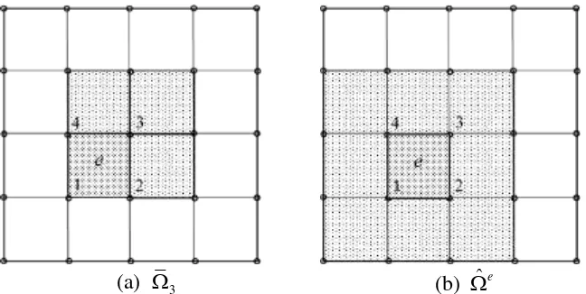
domain of node 3 of element e is shown in Fig. 1(a). The element support 100

domain ˆeis then defined as the union of the four nodal support 101

domains, that is,    ˆe 4_{1 i}, as shown in Fig. 1(b). 102

Consider a nodal support domain of node i, _i with the total number of 103

supporting nodes n. Let the labels for the nodes be j, j=1,…, n. Using the 104

least-squares method, the nodal approximation ui(x,y) is given as 105

T 1

( , ) ( , )

i

u x y p x y A Ba (3)

106

where p(x, y) is a vector of polynomial basis functions, viz. 107





T 2 2

( , )x y  1 x y x xy y

p (1m) (4)

(a) ₃ (b) ˆe

Figure 1 Definitions of: (a) the nodal support domain of node 3 of element e

109

and (b) the element support domain of element e. 110

Here m is the number of monomial bases in p. Following the original 111

work [6], in this study the ‘serendipity’ basis function 112





T 2 2 2 2

( , )x y  1 x y x xy y x y xy

p is used if n8 and the

bi-113

linear basis function pT( , )x y 



1 x y xy



is used if n8. Matrices A 114

and B are the moment matrix and the basis matrix, respectively, given as 115

T 1 ( , ) ( , ) n

j j j j j x y x y 



A p p (m m ) (5)

116



( , )x y1 1 ( ,x y2 2) ( ,x yn n)





B p p p (m n ) (6)

117

Vector a



a1 a2 an



Tis the vector of nodal parameters. Note that 118

in general vector a is not a vector of nodal values because the 119

approximation ui(x,y) does not necessarily pass through the nodal values. 120



f x y g x y( , ), ( , )







n_j1f x y g x y( ,j j) ( ,j j) (7)

122

and using the Gram-Schmidt orthonormalization algorithm [6], the basis 123

vector p can be transformed into an orthonormal basis function vector r 124

so that the moment matrix A becomes the identity matrix. Subsequently, 125

the nodal approximation is constrained using the Lagrange multiplier 126

method so that the nodal parameter ui(x,y) at node i is equal to the nodal 127

value ui. Going through the abovementioned process, the nodal 128

Consider now the element support domain of element e, ˆe, with the

(1), the approximate function can be expressed as 141

the element support domain. In this equation, if node I is not in the nodal 144

support domain of node i, then i( , )

I x y

 is defined to be zero. It is obvious 145

that the shape function is the product of the nonconforming rectangular 146

examined. To measure the approximation errors, the following relative L2

154

2

using Gaussian quadrature rule. The number of quadrature sampling 162

points is taken to be 5 5 . For the purpose of comparison, the accuracy 163

and convergence of the standard Q4 interpolation and its partial 164

derivatives are also presented. 165

3.1 Shape function consistency property 166

In order to be applicable as the basis functions in the Rayleigh-Ritz based 167

numerical method, a set of shape functions is required to be able to 168

represent exactly all polynomial terms of order up to m in the Cartesian 169

coordinates [13], where m is the variational index (that is, the highest 170

order of the spatial derivatives that appears in the problem functional). A 171

set of shape functions that satisfies this condition is called m-consistent 172

(that is, as the mesh is refined, the solution approaches to the exact 174

solution of the corresponding mathematical model). 175

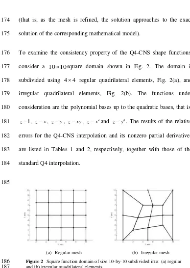
To examine the consistency property of the Q4-CNS shape functions, 176

consider a 10 10 square domain shown in Fig. 2. The domain is 177

subdivided using 4 4 regular quadrilateral elements, Fig. 2(a), and 178

irregular quadrilateral elements, Fig. 2(b). The functions under 179

consideration are the polynomial bases up to the quadratic bases, that is, 180

1

z , zx, z y, zxy, 2

zx and 2

z y . The results of the relative 181

errors for the Q4-CNS interpolation and its nonzero partial derivatives 182

are listed in Tables 1 and 2, respectively, together with those of the 183

standard Q4 interpolation. 184

185

(a) Regular mesh (b) Irregular mesh

Figure 2 Square function domain of size 10-by-10 subdivided into: (a) regular 186

and (b) irregular quadrilateral elements. 187

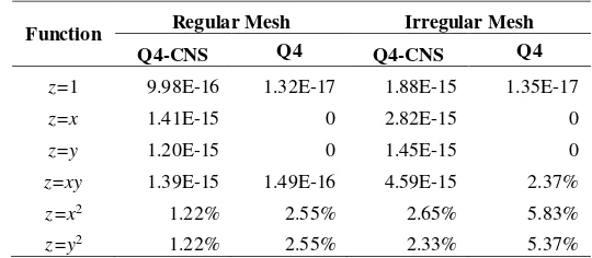
Table 1 Relative L2 norm of errors for the approximation of different 189

polynomial basis functions using the regular and irregular meshes. 190

Function Regular Mesh Irregular Mesh

Q4-CNS Q4 Q4-CNS Q4

Table 2 Relative L2 norm of errors for the approximation of nonzero 192

polynomial basis function derivatives using the regular and irregular 193

meshes. 194

(a) Basis function derivatives with respect to x

195

Function Derivative to

x

Regular Mesh Irregular Mesh

Q4-CNS Q4 Q4-CNS Q4

z,x=1 9.11E-15 2.25E-16 2.15E-14 2.82E-16 z,x=y 9.36E-15 2.55E-16 3.06E-14 11.32% z,x=2x 6.70% 12.50% 10.94% 16.58%

(b) Basis function derivatives with respect to y

196

Function Derivative to

y

Regular Mesh Irregular Mesh

Q4-CNS Q4 Q4-CNS Q4

irregular meshes. In other words, the Q4-CNS interpolation is consistent 200

up to the same basis for the regular mesh, but it is only purely linear 202

consistent for the irregular mesh. This finding may partly explain the 203

reason the Q4-CNS has higher tolerance to mesh distortion [6]. For the x2

204

and y2 bases, both the Q4-CNS and Q4 interpolations are not able to 205

produce the exact solutions, as expected. For these bases, the Q4-CNS 206

interpolation is consistently more accurate than the standard Q4. 207

The tables clearly reveals that the Q4-CNS interpolation is not consistent 208

up to all of the quadratic bases. As a consequence, the Q4-CNS is not 209

applicable to variational problems possessing variational index m=2, 210

including the Love-Kirchhoff plate bending and shell models. This is in 211

contradiction to the statement made in the original paper [6], which 212

mentioned that the Q4-CNS “is potentially useful for the problems of 213

bending plate and shell models”. If the Reissner-Mindlin theory is 214

adopted, however, the Q4-CNS is of course applicable. 215

3.2 Accuracy and Convergence 216

3.2.1 Quadratic function 217

The accuracy and convergence of the Q4-CNS interpolation in fitting 218

functions in 2D domain are firstly examined using quadratic function 219

2 2

1

z x y (16)

221

with two different domains, viz. 222





S ( , ) 0x y x 1, 0 y 1

      (17)

223



2 2



C ( , )x y x y 1,x 0,y 0

      (18)

224

The first domain, Eqn. (17), is the unit square while the second one, Eqn. 225

(18), is a quarter of the unit circle, both of which are located in the first 226

quadrant of the Cartesian coordinate system. The unit square is 227

subdivided using regular meshes of 2 2 , 4 4 , 8 8 , and 16 16 square 228

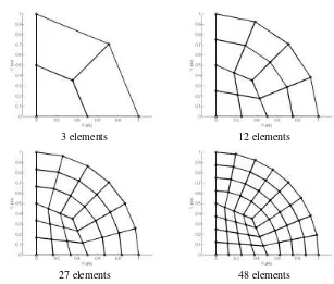
elements. The quarter of the unit circle is subdivided into 3, 12, 27, and 229

48 quadrilateral elements as shown in Fig. 3 (taken from an example in 230

Katili [15]). 231

The relative error norms of the Q4-CNS and Q4 interpolations in 232

approximating the quadratic function, Eqn. (16), and its partial 233

derivatives, are presented in Table 3 for the square domain and in Table 4 234

for the quarter circle domain. The tables show that the Q4-CNS 235

interpolation converges very well to the quadratic function z both for the 236

regular mesh in the unit square domain and for the relatively irregular 237

mesh in the quarter of the unit circle domain. The tables also confirm that 238

interpolation. The finer the mesh the more accurate the Q4-CNS 240

interpolation compared to the Q4. 241

242

3 elements 12 elements

27 elements 48 elements

Figure 3 A quarter of the unit circle subdivided into different number of 243

quadrilateral elements (Katili [15], p.1899). 244

245

Table 3 Relative L2 norm of errors for the approximation of the quadratic 246

function, rz, and its partial derivatives, rz,x and rz,y over the unit square

247

domain. 248

M rz rz,x rz,y

Q4-CNS Q4 Q4-CNS Q4 Q4-CNS Q4

2 10.18% 16.26% 22.77% 25.00% 26.29% 28.87%

4 1.83% 4.07% 10.62% 12.50% 12.26% 14.43%

8 0.33% 1.02% 4.13% 6.25% 4.77% 7.22%

16 0.06% 0.25% 1.52% 3.13% 1.76% 3.61%

Table 4 Relative L2 norm of errors for the approximation of the quadratic 249

function, rz, and its partial derivatives, rz,x and rz,y over a quarter of the

250

unit circle domain. 251

Number of elements

rz rz,x rz,y

Q4-CNS Q4 Q4-CNS Q4 Q4-CNS Q4

3 11.06% 16.59% 28.14% 33.92% 22.48% 27.10% 12 2.51% 4.52% 14.56% 16.16% 12.57% 13.96%

27 0.91% 2.04% 8.42% 10.68% 7.37% 9.36%

48 0.44% 1.15% 5.64% 7.99% 4.97% 7.03%

252

253

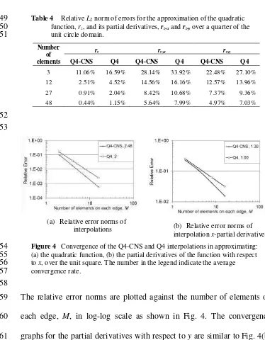
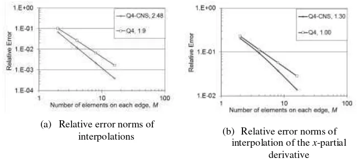
(a) Relative error norms of

interpolations (b) Relative error norms of interpolation x-partial derivative Figure 4 Convergence of the Q4-CNS and Q4 interpolations in approximating: 254

(a) the quadratic function, (b) the partial derivatives of the function with respect 255

to x, over the unit square. The number in the legend indicate the average 256

convergence rate. 257

258

The relative error norms are plotted against the number of elements on 259

each edge, M, in log-log scale as shown in Fig. 4. The convergence 260

graphs for the partial derivatives with respect to y are similar to Fig. 4(b) 261

and have the same convergence rates. The graphs show that the average 262

convergence rate of the Q4-CNS interpolation is about 25% faster than 263

the Q4 interpolation, 2, and its partial derivatives, 1, are exactly the same 265

as predicted by the interpolation theory [16]. 266

3.2.2 Cosine function 267

The second function chosen to examine the accuracy and convergence of 268

the Q4-CNS interpolation is 269

cos( ) cos( )

2 2

z x  y (19)

270

defined over the square unit domain, Eqn. (17). The meshes used are the 271

same as those in the previous example. 272

The convergence graphs of the relative error norms of the Q4-CNS and 273

Q4 interpolations and their partial derivatives with respect to x are shown 274

in Fig. 5. The graphs confirm the superiority of the Q4-CNS interpolation 275

over the Q4 interpolation both in terms of the accuracy and convergence 276

rate. 277

4 Conclusions 278

The consistency property, accuracy and convergence of the Q4-CNS 279

interpolation in surface fitting problems have been numerically studied. 280

The results show that the Q4-CNS interpolation is consistent up to the 281

bilinear basis both for the regular and irregular meshes. It is more 282

sufficiently fine mesh, the error norm of the Q4-CNS interpolation is 284

around 3 to 4 times smaller than that of the Q4, and the error norm of its 285

derivatives is around 1.5 to 2 times smaller than that of the Q4. The Q4-286

CNS interpolation converge very well to the fitted function. Its 287

convergence rate is approximately 25% faster than that of the Q4. The 288

demerits of the present method is that the computational cost to construct 289

the shape function is much higher than the Q4 shape function. 290

291

(a) Relative error norms of

interpolations (b) Relative error norms of interpolation of the x-partial

derivative Figure 5 Convergence of the Q4-CNS and Q4 interpolations in approximating: 292

(a) the bi-cosine function, (b) the partial derivatives of the function with respect 293

to x, over the unit square. The number in the legend indicate the average 294

convergence rate. 295

296

297

Acknowledgement 299

We gratefully acknowledge that this research is partially supported by the 300

research grant of the Institute of Research and Community Service, Petra 301

Christian University, Surabaya. 302

5 References 303

[1] Liu, G.R., Mesh Free Methods: Moving Beyond the Finite Element

304

Method, 1st ed., Boca Raton: CRC Press, 1-5, 2003. 305

[2] Gu, Y.T., Meshfree Methods and Their Comparisons, International 306

Journal of Computational Methods, 2(4), pp. 477–515, 2005. 307

[3] Liu, G.R., An Overview on Meshfree Methods: For Computational

308

Solid Mechanics, International Journal of Computational Methods, 309

13(5), pp. 1630001-1–1630001-42, 2016. 310

[4] Rajendran, S. & Zhang, B.R., A ‘FE-meshfree’ Q4 Element Based

311

on Partition of Unity, Computer Methods in Applied Mechanics 312

and Engineering, 197(1–4), pp. 128–147, 2007. 313

[5] Zhang, B.R. & Rajendran, S., ‘FE-meshfree’ Q4 Element for

Free-314

vibration Analysis, Computer Methods in Applied Mechanics and 315

[6] Tang, X.H., Zheng, C., Wu, S.C., & Zhang, J.H., A Novel

Four-317

node Quadrilateral Element with Continuous Nodal Stress, Applied 318

Mathematics and Mechanics, 30(12), pp. 1519–1532, 2009. 319

[7] Yang, Y., Tang, X.H., & Zheng, H., A Three-node Triangular

320

Element with Continuous Nodal Stress, Computers & Structures, 321

141, pp. 46–58, 2014. 322

[8] Yang, Y., Bi, R., & Zheng, H., A Hybrid ‘FE-meshless’ Q4 with

323

Continuous Nodal Stress using Radial-polynomial Basis Functions, 324

Engineering Analysis with Boundary Elements, 53, pp. 73–85, 325

2015. 326

[9] Yang, Y., Chen, L., Xu, D., & Zheng, H., Free and Forced

327

Vibration Analyses using the Four-node Quadrilateral Element

328

with Continuous Nodal Stress, Engineering Analysis with 329

Boundary Elements, 70, pp. 1–11, 2016. 330

[10] Yang, Y., Sun, G., Zheng, H., & Fu, X., A Four-node

331

Quadrilateral Element Fitted to Numerical Manifold Method with

332

Continuous Nodal Stress for Crack Analysis, Computers & 333

Structures, 177, pp. 69–82, 2016. 334

[11] Yang, Y., Chen, L., Tang, X.H., Zheng, H., & Liu, Q.S., A

335

Partition-of-unity Based ‘FE-meshfree’ Hexahedral Element with

Continuous Nodal Stress, Computers & Structures, 178, pp. 17–28, 337

2017. 338

[12] Zienkiewicz, O.C. & Taylor, R.L., The Finite Element Method,

339

Volume 2: Solid Mechanics, 5th ed., Butterworth-Heinemann, 126, 340

2000. 341

[13] Felippa, C.A., Introduction To Finite Element Methods (ASEN

342

5007), Fall 2016 , University of Colorado at Boulder, 343

http://www.colorado.edu/engineering/cas/courses.d/IFEM.d/, (14-344

Oct-2016). 345

[14] Wong, F. T. & Kanok-Nukulchai, W., Kriging-based Finite

346

Element Method : Element-by-Element Kriging Interpolation, Civil 347

Engineering Dimension, 11(1), pp. 15–22, 2009. 348

[15] Katili, I., A New Discrete Kirchhoff-Mindlin Element based on

349

Mindlin-Reissner Plate Theory and Assumed Shear Strain Fields-

350

Part II: an Extended DKQ Element for Thick-Plate Bending

351

Analysis, International Journal for Numerical Methods in 352

Engineering, 36(11), pp. 1885–1908, 1993. 353

[16] Bathe, K.J., Finite Element Procedures, Prentice-Hall, 244-250, 354