Ileana-Rotar-Incse. 214KB Jun 04 2011 12:09:02 AM

THE OPTIMIZATION OF FEED FORWARD NEURAL

NETWORKS STRUCTURE USING GENETIC

ALGORITHMS

by

Ioan Ileană, Corina Rotar, Arpad Incze

Keywords: feed-forward neural networks, layers, back propagation, genetic algorithms.

1. Introduction

Artificial neural networks (RNAs) are an interesting approach in solving some difficult problems like pattern recognition, system simulation, process forecast etc. The artificial neural networks have the specific feature of “storing” the knowledge in the synaptic weights of the processing elements (artificial neurons). There are a great number of RNA types and algorithms allowing the design of neural networks and the computing of weight values.

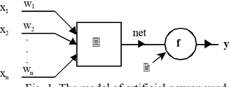
In this paper we present several results related to optimization of feed-forward neural networks structure by using genetic algorithms. Such a network must satisfy some requirements: it must learn the input data, it must generalize and it must have the minimum size allowed to accomplish the first two tasks. The processing element of this type of network is shown in figure 1.

Fig. 1. The model of artificial neuron used

The output of the neuron may be written:

y = f (net-2) = f (wTx-2) (2)

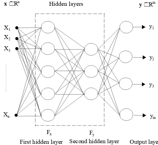
In practical applications, the neural networks are organized in several layers as shown in figure 2.

2. Design approaches for feed-forward neural networks

Implementing a RNA application implies three steps [3]:

• Choice of network model;

• Correct dimensioning of the network;

• The training of the network using existing data (synaptic weights synthesis).

The present paper is dealing with feed-forward neural network so we concentrate on steps 2 and 3.

Network dimension must satisfy at least two criteria:

• The network must be able to learn the input data ;

• The network must be able to generalize for similar input data that were not in training set.

Hidden layers

X1 X2

X3

Xn

Fx

First hidden layer

Fy

Second hidden layer Output layer

x Rn

y Rm

y1

y2

y3

ym

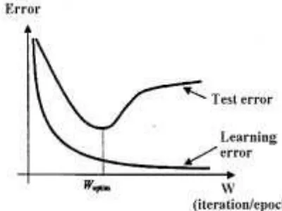
The accomplishment degree of these requirements depends on the network complexity and the training data set and training mode. Figure 3 shows the dependence of network performance in function of the complexity and figure 4 shows the same dependence of the training mode.

Fig. 3. Performance’s dependence of network complexity. Source: [3], p. 74.

Fig. 4. Performance’s dependence of the training mode. Source: [6], p. 40.

One can notice that the two requests are contradictory and that the establishment of the right dimension is a complex matter. We generally wish to diminish the complexity of the model, which leads to a better generalization, to an increased training speed and to lower implementation cost.

dimension implies the establishment of the layer number, neuron number in each layer and interconnections between neurons. At the time being, there are no formal methods for optimal choice of the neural network’s dimensions.

The choice of the number of layers is made knowing that a two layer network (one hidden layer) is able to approximate most of the non linear functions demanded by practice and that a three layer network (two hidden layers) can approximate any non linear function. Therefore it would result that a three layer network would be sufficient for any problem. In reality the use of a large number of hidden layers can be useful if the number of neurons on each layer is too big in the three layer approach.

Concerning the dimension of each neuron layer the situation is as follows:

• Input and output layers are imposed by the problem to be solved;

• The dimension of hidden layers is essential for the efficiency of the network and there is a multitude of dimensioning methods (table 1). Table 1. Source: [3] p. 86.

Hidden layer dimensioning methods Type of method

Empirical methods Direct

Methods based on statistic criteria Indirect

Constructive Direct Destructive Direct Mixed Direct Ontogenic methods

Based on Genetic

Algorithms Direct

Most methods use a constructive approach (one starts with a small number of neurons and increases it for better performances) or a destructive approach (one starts with a large number of neurons and drops the neurons with low activity).

3. The proposed approach

As we have previously seen, optimal designing of feed forward neural networks is a complex problem and three criterions must be satisfied:

• The network must have the capacity of learning

• The network must have the capacity of generalization

• The network must have the minimum number of neurons.

Next we shall present one method of optimizing the network’s structure, by the use of Genetic Algorithms (GA). Genetic algorithms proved their efficiency in solving optimization problems and, moreover, many evolutionary techniques have been developed for determining multiple optima of a specific function.

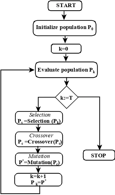
According to the evolutionary metaphor, a genetic algorithm starts with a population (collection) of individuals, which evolves toward optimum solutions through the genetic operators (selection, crossover, mutation), inspired by biological processes [2].

Each element of the population is called chromosome and codifies a point from the search space. The search is guided by a fitness function meant to evaluate the quality of each individual. The efficiency of a genetic algorithm is connected to the ability of defining a “good” fitness function. For example, in real function optimization problems, the fitness function could be the function to be optimized. The standard genetic algorithm is illustrated in the figure 2.

Multicriteria optimization

The multicriteria optimization (multi-objective optimization or vector optimization) may be stated as follows: the vector:



that satisfies the constraints:

( )

x ≥0

( )

( )

( )

must be determined, where x represents the vector of decision variables. In other words we want to find from the set F of the values that satisfy (1) and (2), the particular values x₁*,x*₂, … , x_n* that produce optimal values for the objective function. In this situation the desired solution would bex*, but there are few situations in which all the f_i

( )

x have minimum (or maximum) in F in a common pointx*. It is necessary to state what “optimal solution” is.

START

Initialize population P0

Evaluate population Pk

k:=T

Pareto optimum

The most popular optimal approach was introduced by Vilfredo Pareto at the end of XIX century: One vector x*∈F of decision variables is Pareto optimal if there isn’t another vector x∈F with properties:

( )

( )

*

This optimality criterion will supply a set of solutions denoted Pareto optimal set. The vectors x* corresponding to the solutions included in Pareto set will be denoted dominants. The area from F formed by the non-dominant solutions makes Pareto front.

Evolutionary approach

For solving the above problem we used two evolutionary approaches: one approach that doesn’t use the concept of Pareto dominance when evaluating candidate solutions (non Pareto method) - weights method - and one Pareto approach recently developed inspired by endocrine system.

Non-Pareto method (Weights method)

The technique of combining all the objective functions in one function is denoted the function aggregation method and the most popular such method is the weights method.

In this method we add to every criterion f_i a positive sub unity value

i

w denoted weight. The multicriteria problem becomes a unicriteria optimization problem

If we want to find the minimum, the problem can be stated as follows:

( )

One drawback of this method is the determination of weights if one don’ know many things about the problem to be solved.

Pareto method

1. One maintains two populations: one active population of individuals (hormones) H, and one passive population of non-dominant solutions T. The members of passive T population act like an elite collection having the function of guiding the active population toward Pareto front and keeping them well distributed in search space.

2. The passive T population doesn’t suffer any modifications at individuals’ level through variation operators like recombining or mutation. In the end the T will contain a previously established number of non-dominating vectors supplying a good approximation of the Pareto front.

3. At each T generation the members of the t

H active population are divided in st classes, where st represents the number of tropes from the current T population. Each hormone class is supervised by a correspondent trope. The point is that each h hormone from

t H is controlled by the nearest a_itrope fromA_t.

4. Two individuals’ evaluation functions are defined. The value of the first one for an individual represents the number of individuals of the current population that are dominated by it. The value of the second function for an individual represents the agglomeratedegree from the class corresponding to that particular individual.

5. The recombining selection takes into consideration the values of the first function as well as the values of the second. The first parent is selected through competition taking into consideration the values of the second performance function. The second parent is selected proportional from the first parent’s class taking into consideration the second performance function.

4. Experimental results

-6,00

Fig. 5. The non linear function approximated by the network

The chromosomes will codify the network dimension (number of layers, number of neurons on layer) and the fitness function will integrate the training error (after a number of 100 epochs), the testing error (as a measure of the generalization capacity) and the entire number of neurons of the network. To simplify we considered only two or three layers networks. The maximum number of neurons on each layer is 10. There is one output neuron. The results obtained are shown in tables 2 and 3.

Table 2.

Weights method Population dimension 20

Number of generations

100

Criteria F1 – training error, F2 – test error, F3 – inverse of neuron number

Technique inspired by endocrine system Population dimension 20

Number of generations

Criteria F1 – training error F2 – test error Solutions: (2,8)

The structure obtained by the use of the optimizing algorithm was tested in Matlab and the results are shown in figures 6 and 7.

5. CONCLUSIONS

The optimal dimensioning of a feed-forward neural network is a complex matter and literature presents a multitude of methods but there isn’t a rigorous and accurate analytical method.

Our approach uses genetic computing for the establishment of the optimum number of layers and the number of neurons on layer, for a given problem. We used for illustration the approximation of a real function with real argument but the method can be used without restrictions for modeling networks with many inputs and outputs.

We intent to use more complex fitness functions in order to include the training speed.

Fig. 6. Output of the 2:8:1 network (+) compared

Fig. 7. Output of the 1:4:1 network (+) compared

with desired output (line)

References:

1. Bäck T., Evolutionary Algorithms in Theory and Practice, Oxford University Press, 1996.

2. Coello C. A.. C., An Updated Survey of Evolutionary Multiobjective Optimization Techniques : State of the Art and Future Trends , In 1999 Congress on Evolutionary Computation, Washington, D.C., 1999.

3. Dumitraş Adriana (1997): Proiectarea reţelelor neuronale artificiale, Casa editorială Odeon, 1997.

4. Dumitrescu D., Lazzerini B., Jain L.C., Dumitrescu A., Evolutionary Computation, CRC Press, Boca Raton London, New York, Washington D.C., 2000.

5. Goldberg D.E., Genetic Algorithms in Search, Optimization, and Machine Learning, Addison-Wesley Publishing Company, Inc., 1989.

6. Năstac Dumitru Iulian: Reţele neuronale artificiale. Procesarea avansată a datelor, Editura Printech, 2002.

8. Rotar C., Ileană I., Models of Population for Multimodal Optimization. A New Evolutionary Approach, Proc. 8th Int. Conf. on Soft Computing, Mendel2002, Czech Republic, 2002.

9. Rotar Corina, A new evolutionary algorithm for multicriterial optimization based on endocrine paradigm, ICTAMI 2003, publicat in Acta Universitatis Apulensis, seria Matematics-Informatics.

10. Rotar Corina, Ileana Ioan, Risteiu Mircea, Joldes Remus, Ceuca Emilian, An evolutionary approach for optimization based on a new paradigm, Proceedings of the 14th international conference Process Control 2003, Slovakia, 2003, pag. 143.1 – 143.8.

Authors: