ON THE TRACE CHARACTERIZATION OF THE JOINT
SPECTRAL RADIUS∗
JIANHONG XU†
Abstract. A characterization of the joint spectral radius, due to Chen and Zhou, relies on the limit superior of thek-th root of the dominant trace over products of matrices of lengthk. In this note, a sufficient condition is given such that the limit superior takes the form of a limit. This result is useful while estimating the joint spectral radius. Although it applies to a restricted class of matrices, it appears to be relevant to many realistic situations.
Key words. Joint spectral radius, Spectral radius, Trace, Primitivity, Nonnegative matrix.
AMS subject classifications.15A18, 15A69, 65F15.
1. Introduction. The joint spectral radius has drawn much attention lately, see, for example, [1, 2, 3, 4, 5, 6, 7, 9, 13, 18] and the references therein, due to its applications in various areas such as switched systems [12], differential equations [8], coding theory [14], and wavelets [15]. For more background material, we also refer the reader to the monograph [11].
As the joint spectral radius can be regarded as a generalization of the (conven-tional) spectral radius, we shall denote throughout both the joint spectral radius
and the spectral radius by ρ(·). It is well known that given a set ofn×n matrices
Σ ={A1, . . . , Am}, its joint spectral radius can be characterized by
ρ(Σ) = lim
k→∞Amax∈Πkk Ak1/k,
(1.1)
with Πk being the set of products of Ai of length kwhose factors are in Σ andk · k
being a matrix norm; or, equivalently, by
ρ(Σ) = lim sup
k→∞ max
A∈Πk
ρ1/k(A).
(1.2)
Recently, Chen and Zhou showed in [4], also see [18], thatρ(Σ) can be expressed
alternatively as
ρ(Σ) = lim sup
k→∞ max
A∈Πk|
tr(A)|1/k.
(1.3)
∗Received by the editors February 14, 2010. Accepted for publication July 9, 2010. Handling
Editor: Michael Neumann.
†Department of Mathematics, Southern Illinois University Carbondale, Carbondale, Illinois 62901,
USA ([email protected]).
This result was then used in [4, 18] to estimateρ(Σ). An attractive feature of (1.3) is
that it characterizesρ(Σ) by the trace, hence it is computationally less expensive1as
compared to (1.1) — assuming here a general subordinate matrix norm — and (1.2).
However, the utilization of (1.3) can be complicated as it involves a limit superior, which implies that, in general, the convergence in (1.3) is attained only on some
subsequence{ki}, whereki→ ∞asi→ ∞. It is therefore natural for us to ask when
the convergence is attained on any subsequence{ki}, i.e. in the sense of a limit.
In this short note, we shall illustrate that the limit superior in (1.3) can be replaced with a limit when Σ is a set of nonnegative matrices which has at least one primitive element. From a computational perspective, this outcome is handy since it
guarantees that with any subsequence{ki}, the corresponding
{max
A∈Πki|
tr(A)|1/ki
}
provides, in general, increasingly tighter approximations toρ(Σ) aski grows.
2. Trace Characterization. Given a matrixA, the notationsA≥0 andA >0
are interpreted in an entrywise sense. Recall that a square matrix A ≥ 0 is called
primitive ifAk >0 for some integerk≥1. In the sequel, matrices are assumed to be
square. Let us begin with the following lemma:
Lemma 2.1. ([17, p.49]) Let A≥0 be primitive. Then
ρ(A) = lim
k→∞tr
1/k(Ak).
(2.1)
We comment that the assumption of primitivity in Lemma 2.1 is necessary.
Con-sider, for instance, A =
0 1
1 0
, which is not primitive; clearly, tr(Ak) = 0 or 2,
depending on whetherkis odd or even, thus the limit in (2.1) does not exist.
Inciden-tally, if A≥0 is irreducible, i.e. its underlying digraph is strongly connected, and if
the diagonal entries ofAare not all zero, thenAmust be primitive. This requirement
on the diagonal entries serves as a convenient, although only sufficient, condition for determining primitivity — note that, conversely, primitivity implies irreducibility.
We shall also need a conclusion from [2] as below.
1Nevertheless, the computation of the joint spectral radius remains a tough challenge since the
main difficulty comes from the cardinality of Πkaskgrows, or the construction of extremal polytope
([2, Theorem 3])LetΣ ={A1, . . . , Am}be a set ofn×nnonnegative
matrices. Then
ρ(Σ) = lim
k→∞ρ
1/k(A⊗k
1 +. . .+A
⊗k m),
whereA⊗k is the k-th Kronecker power ofA.
For background material on the Kronecker power and, more generally, Kronecker product, see [10, 16]; a few properties of such products are used in this note without being first stated as preparatory lemmas. However, we mention here that, according to [10, Lemma 4.2.10], it follows by induction that
A⊗1k· · ·Al⊗k= (A1· · ·Al)⊗k
(2.2)
holds for any positive integerskandl. In particular, (A⊗k)l= (Al)⊗k.
Continuing, we point out that applying Lemma 2.1, along with Lemma 2.2, to answer our main question here hinges on the next two simple, yet useful, observations.
Lemma 2.3. Suppose that A ≥ 0 is primitive. Then A⊗k is also primitive for
any integerk≥1.
Proof. By the assumption, there exists some integer l ≥ 1 such that Al > 0.
Hence
(A⊗k)l= (Al)⊗k >0.
This completes the proof.
We mention in passing that Lemma 2.3 does not extend to irreducibility of
ma-trices. Consider, again,A=
0 1 1 0
,which is indeed irreducible; but it is easy to
verify that, for example,A⊗2 is no longer irreducible.
Lemma 2.4. Suppose that {A1, . . . , Am} is a set of nonnegative matrices of the
same size, where at least oneAi is primitive. Then A1+. . .+Amis also primitive.
Proof. Without loss of generality, we assume thatA1 is primitive. Thus there
exists an integerk≥1 such thatAk
1 >0. We notice that
(A1+. . .+Am)k≥Ak1 >0,
which yields the conclusion.
We are now ready to state the following result:
Theorem 2.5. For a set Σ ={A1, . . . , Am}of n×nnonnegative matrices, with
at least oneAi being primitive,
ρ(Σ) = lim
k→∞Amax∈Πk
tr1/k(A),
whereΠk is the set of products ofAi of lengthk whose factors are in Σ.
Proof. First of all, based on Lemmas 2.3 and 2.4,A⊗1k+. . .+A⊗k
m is primitive
for anyk. Therefore, Lemma 2.1 may be exploited to formulateρ(A⊗1k+. . .+A⊗k
m ).
For any integersk, l≥1, we observe that, using (2.2),
tr A⊗1k+. . .+A⊗k m
l
= trP
1≤i1,...,il≤mA ⊗k
i1 · · ·A⊗ilk
= trhP
1≤i1,...,il≤m(Ai1· · ·Ail) ⊗ki
= P
1≤i1,...,il≤mtr (Ai1· · ·Ail) ⊗k
= P
1≤i1,...,il≤mtrk(Ai1· · ·Ail),
i.e.
tr A⊗1k+. . .+A⊗mk
l
= X
A∈Πl
trk(A),
(2.4)
with the cardinality of Πlbeing N=ml. Obviously, (2.4) implies
tr1/kl A⊗1k+. . .+A⊗mk
l
≤m1/kmax
A∈Πl
tr1/l(A).
(2.5)
Assumingσ(A⊗1k+. . .+A⊗k
m ) ={λ1, . . . , λnk}, whereσ(·) denotes the spectrum,
we arrive at
tr(A⊗1k+. . .+Am⊗k)l=λl1+. . .+λ
l
nk ≤nkρl(A⊗k
1 +. . .+A
⊗k m ),
which, together with (2.4), leads to
max
A∈Πl
tr1/l(A)≤tr1/kl A⊗k
1 +. . .+A⊗mk
l
≤n1/lρ1/k(A⊗k
1 +. . .+A⊗mk).
(2.6)
It now follows from (2.5) and (2.6) that for any integersk, l≥1,
tr1/kl A⊗k
1 +. . .+A⊗mk
l
m1/k ≤Amax∈Πltr
1/l(A)
≤n1/lρ1/k(A⊗k
1 +. . .+A
⊗k m ).
(2.7)
By taking the iterated limit limk→∞liml→∞ in the above inequalities and resorting
to Lemmas 2.1 and 2.2, we conclude that
lim
k→∞llim→∞Amax∈Πl
tr1/l(A) =ρ(Σ),
Concerning Theorem 2.5, we remark that in view of the previous 2×2 example,
(2.3) may fail without the primitivity ofAi’s — if so, the limit superior formulation
is required in (2.3). However, in its proof, we see that primitivity is needed merely in the left inequality of (2.7). In other words, Theorem 2.5 still holds if its assumption is
relaxed to the primitivity ofA⊗1k+. . .+A⊗k
m at anyk. For example, take Σ ={A1, A2},
where
A1=
0 1
1 0
and A2=
1 1
0 1
,
neither being primitive. It can be readily verified that when l ≥ 4, either S =
l/2
Y
i=1
(A1A2)>0 for any even lor T =A1·
⌊l/2⌋ Y
i=1
(A2A1)>0 for any oddl, where⌊·⌋ is
the floor function. But then
(A⊗1k+A⊗2k)l= X
1≤i1,...,il≤2
(Ai1· · ·Ail)⊗k,
which implies that (A⊗1k+A⊗2k)l is no less thanS⊗k or T⊗k, depending on whether
l is even or odd. ThusA⊗1k+A⊗2k is primitive for allk. In other words, Theorem 2.5
remains valid on the set Σ ={A1, A2}.
Our second observation from Theorem 2.5 is the following estimate ofρ(Σ), which
arises as we pushl→ ∞in (2.7):
Corollary 2.6. (see also [2, Theorem 3]) Under the same assumption as in
Theorem 2.5,
ρ1/k A⊗k
1 +. . .+A⊗mk
m1/k ≤ρ(Σ)≤ρ1 /k(A⊗k
1 +. . .+A
⊗k m )
(2.8)
for any integerk≥1.
While being free of products ofAi’s, one drawback of (2.8) is the huge size of the
eigenproblem being involved. When n= 2, for example, a case with k = 15 would
exhaust the available memory on a typical modern PC platform.
As we mentioned earlier, the trace characterization is computationally more ad-vantageous than that in (1.1) or (1.2). It is also known that the trace operator is
invariant under cyclic shifts of the factors in a product ofAi’s. However, the benefit
from this invariance is limited. Consider all products ofAi’s of length k. Let ki be
the number of Ai’s. Then for each fixed set of {k1, . . . , km}, there are
k!
k1!· · ·km!
different arrangements of the factors, while under the cyclic-shift equivalence, this
number is reduced by a factor ofk to 1
k· k!
k1!· · ·km!
are effectively a total ofm /k different arrangements ofAi’s of lengthk. Clearly, the
reduction is not significant as compared with mk.
In addition, it is interesting to note that (2.1) can now be thought of as a special
case of (2.3) when the set Σ consists of a single elementA. Such an extension of (2.1)
is parallel to that from the well-known Gelfand’s formula
ρ(A) = lim
k→∞kA k
k1/k
to formula (1.1).
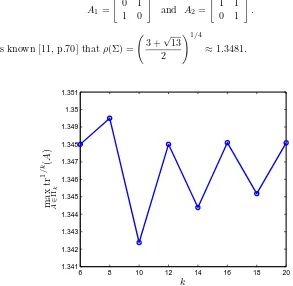
Finally, we give an example which implements (2.3) in Matlab. Again, set Σ =
{A1, A2}, where
A1=
0 1
1 0
and A2=
1 1 0 1
.
It is known [11, p.70] thatρ(Σ) = 3 +
√
13 2
!1/4
≈1.3481.
6 8 10 12 14 16 18 20
1.341 1.342 1.343 1.344 1.345 1.346 1.347 1.348 1.349 1.35 1.351
k
m
ax
A
∈
Π
k
tr
1
/
k (
A
[image:6.612.86.379.316.602.2])
Fig. 2.1.The curve representsmaxA∈Πktr1
/k(A), which approachesρ(Σ)askincreases. The
computation is carried out in Matlab on a Dell Precision workstation with dual Xeon CPU’s at
3.0GHz and2 GB RAM. The total running time is approximately250seconds with four pools in
Matlab’s Parallel Computing Toolbox.
Consider next possible arrangements ofAi’s of length k. Any such arrangement
A2, respectively. All such words can be obtained by calling de2bi(0:2^k-1,k,2).
The result is a 2k×k array, denoted here byu, where each row translates to a word
— we choose to generate the words at once without using a loop for the sake of speed.
For the same reason, the arrangement corresponding to wordu(i,:)are constructed
by
kron(1-u(i,:),A_1)+kron(u(i,:),A_2),
which produces a 2×2k array, with all the factors being arranged in this array as
2×2 blocks. Finally, the product of these factors is computed by using a loop. The
numerical result on maxA∈Πktr1
/k(A) is shown in Figure 2.1, while the Matlab code
for this experiment are given in Appendix A.
We mention that the above vectorized implementation runs faster than loops, but it consumes a large amount of memory. To address this issue, we may generate one
u(i,:)at a time — the trade-off, of course, is the loss of speed.
3. Concluding Remarks. It is demonstrated here the limit superior in (1.3) can be replaced by a limit under certain circumstances. Particularly, the presence of primitivity turns out to be a sufficient condition. The lack of premitivity generally entails the limit superior formulation.
The significance of this result lies in the fact that maxA∈Πktr1
/k(A) now
ap-proachesρ(Σ) from both above and below. Accordingly, any subsequence of{k}may
be used to estimateρ(Σ) with the trace characterization. Seeing the role that
nonneg-ative matrices play in many applications, we feel that this note is relevant to tackling problems which involve the joint spectral radius.
The trace characterization as in (2.3) can be efficiently implemented in Matlab as shown by the numerical example. Even though the applicability of this method is largely limited by the nature of the joint spectral radius, the approach we discuss here appears to be useful for solving small-scale problems concerning the joint spectral radius as well as for estimating this crucial quantity for problems of larger size by
resorting to smallerk-values in (2.3).
Appendix A. Matlab Code.
%estimating joint spectral radius with trace characterization clear all
a1=[0 1; 1 0]; a2=[1 1; 0 1]; k=6:2:20; m=length(k);
%matlabpool open 4 %parallel computing toolbox with 4 labs for i=1:m %parfor i=1:m %with parallel computing toolbox
trmax=0; n=2^k(i);
arr=de2bi(0:n-1,k(i),2); %all zero-one words for j=1:n
a=kron(1-arr(j,:),a1)+kron(arr(j,:),a2); u=1:2; %product
p=a(:,u); for v=2:k(i)
u=u+2; p=p*a(:,u); end
tr=trace(p); %trace of product if tr>trmax
trmax=tr; end
end
jsr(i)=trmax^(1/k(i)); end
%matlabpool close %with parallel computing toolbox plot(k,jsr,’-bo’,’LineWidth’,2)
REFERENCES
[1] M. A. Berger and Y. Wang. Bounded semigroups of matrices.Linear Algebra Appl., 166:21–27, 1992.
[2] V. D. Blondel and Y. Nesterov. Computationally efficient approximations of the joint spectral radius.SIAM J. Matrix Anal. Appl., 27:256–272, 2005.
[3] V. D. Blondel, J. Theys, and A. A. Vladimirov. An elementary counterexample to the finiteness conjecture.SIAM J. Matrix Anal. Appl., 24:963–970, 2003.
[4] Q. Chen and X. Zhou. Characterization of joint spectral radius via trace.Linear Algebra Appl., 315:175–188, 2000.
[5] I. Daubechies and J. C. Lagarias. Sets of matrices all infinite products of which converge.Linear
Algebra Appl., 161:227–263, 1992.
[6] I. Daubechies and J. C. Lagarias. Corrigendum/addendum to: Sets of matrices all infinite products of which converge.Linear Algebra Appl., 327:69–83, 2001.
[7] L. Elsner. The generalized spectral radius theorem: An analytic-geometric proof.Linear Algebra
Appl., 220:151–159, 1995.
[8] N. Guglielmi and M. Zennaro. On the zero-stability of variable stepsize multistep methods: the spectral radius approach.Numer. Math., 88:445–458, 2001.
[10] R. A. Horn and C. R. Johnson.Topics in Matrix Analysis. Cambridge University Press, Cam-bridge, 1991.
[11] R. Jungers.The Joint Spectral Radius: Theory and Applications. Springer-Verlag, Berlin, 2009. [12] V. S. Kozyakin. Structure of extremal trajectories of discrete linear systems and the finiteness
conjecture.Automat. Remote Control, 68:174–209, 2007.
[13] J. C. Lagarias and Y. Wang. The finiteness conjecture for the generalized spectral radius of a set of matrices.Linear Algebra Appl., 214:17–42, 1995.
[14] B. Moision, A. Orlitsky, and P. H. Siegel. On codes with local joint constraints.Linear Algebra
Appl., 422:442–454, 2007.
[15] V. Y. Protasov. Fractal curves and wavelets. Izv. Ross. Akad. Nauk Ser. Mat., 70:123–162, 2006.
[16] C. F. Van Loan. The ubiquitous Kronecker product.J. Comput. Appl. Math., 123:85–100, 2000. [17] R. S. Varga,Matrix Iterative Analysis, 2nd ed. Springer-Verlag, Berlin, 2000.