A COMBINED MONTE CARLO AND QUASI-MONTE CARLO METHOD WITH APPLICATIONS TO OPTION PRICING
Natalia C. Ros¸ca
Abstract. In this paper, we apply a combined Monte Carlo and Quasi-Monte Carlo method, which we proposed in an earlier paper [32], to the evaluation of an European Call option and of an Asian Call option. We assume that the stock price of the underlying assetS =S(t) is driven by a L´evy processZ(t), with independent in-crements distributed according to a NIG distribution. We compare our method with the Monte Carlo and Quasi-Monte Carlo methods. The numerical results indicate that our method provides significant error reduction over these methods.
2000Mathematics Subject Classification: 11K36, 11K38, 11K45, 62P05, 65C05, 91B24, 91B28.
Keywords and phrases: Monte Carlo integration, Quasi-Monte Carlo integration,
G-discrepancy, sequences with low G-discrepancy, normal inverse Gaussian distri-bution, option pricing.
1. Introduction
The evaluation of the European and Asian options is one of the most important problems in financial mathematics. The value of such an option can be expressed in terms of a risk-neutral expectation of a random payoff. In the case of European options, when the asset is modeled under the standard Black-Scholes assumptions, the expectation is explicitly computable. However, in general, if the log-returns of the asset prices are non-normally distributed, a closed expression for the price of an European option is not available, and so numerical methods are involved. In the case of arithmetic Asian options, even in the standard Black-Scholes framework, exact closed-form formulas for pricing such options have not been available and therefore, the price must be numerically computed.
MC methods in this field appeared in Boyle [2], who used simulation to estimate the value of a standard European option. Applications of the QMC method to option pricing problems can be found in [8], [14] and [17]. Majority of the work done on applying these simulation techniques to financial problems was in direction where one needs to simulate from the normal distribution.
Barndorff-Nielsen [1] was the one who proposed to model the log-returns, by using the normal inverse Gaussian (NIG) distribution, as this class of distributions has proven to fit the semi-heavily tails observed in financial time series of various kinds extremely well [7], [34]. A method for evaluating such derivatives is the one proposed by Raible [27], who considered a Fourier method to evaluate call and put options. Other alternative methods for evaluating such derivatives are the MC and QMC methods. In [15], Kainhofer proposes a QMC algorithm for generating NIG variables, based on a technique proposed by Hlawka and M¨uck [12, 13] for generating low-discrepancy sequences for general distributions.
In an earlier paper [32], we proposed a combined MC and QMC method, to estimate a multidimensional integral I of a function f, with respect to the proba-bility measure induced by a distribution functionGon [0,1]s. Our method is based on random sampling from sequences with low G-discrepancy. Other methods that combine the ideas of MC and QMC methods and their applications to option pricing can be found in [19], [20], [22], [28], [9] and [29].
In this paper, we first recall the general setting of our combined method and give some important theoretical results. Next, we apply our method to the evalua-tion of an European Call opevalua-tion and of an Asian Call opevalua-tion. We assume that the stock price of the underlying asset S=S(t) is driven by a L´evy process Z(t), with independent increments distributed according to a NIG distribution. We compare the estimate produced by our method with the estimates given by MC and QMC methods. The numerical results indicate that our method provides significant error reduction over these methods.
2. Monte Carlo and Quasi-Monte Carlo methods
We consider ans-dimensional continuous distribution on [0,1]s, with distribution function Gand density functiong (g is nonnegative andR[0,1]sg(u)du= 1).
We consider the problem of approximating the multidimensional integral of a function f : [0,1]s→R, of the form
I = Z
[0,1]s
f(x)dG(x) = Z
[0,1]s
In the MC method, we generate N independent sample variables X1, . . . , XN, with the density function g on [0,1]s. The integral I is estimated by the sample mean
¯
IM C= 1
N
N X
k=1
f(Xk).
The estimator ¯IM C is an unbiased estimator of the integral I. The strong law of large numbers tells us that
P lim N→∞
¯
IM C=I
= 1.
In other words, the MC estimator converges almost surely toI, asN → ∞.
The practical advantage of the MC method is that we can easily measure the accuracy of the MC estimate, by constructing confidence intervals for I. They use the sample standard deviation ¯σ[f] =
q 1 N−1
PN
i=1 f(Xi)−I¯M C 2
, and are of the form [33]
¯
IM C−tN−1,1−α2
¯
σ[f]
√
N,
¯
IM C+tN−1,1−α2
¯
σ[f]
√
N
,
wheretN−1,1−α2 is the 1−α2
-th percentile of the Student’st-distribution withN−1 degrees of freedom, and 1−α is a given confidence level, α∈(0,1).
In the MC method, by constructing confidence intervals forI, we get probabilistic error bounds of order O 1/√N.
The QMC method can be defined by analogy with the MC method, by replacing the random samples by a sequence of ”well distributed” deterministic points. This approach uses the so-called sequences with low G-discrepancy in [0,1]s. We define these sequences, using the notions of G-star discrepancy and G-discrepancy.
Definition 1 (G-star discrepancy). We consider a distribution on [0,1]s,
with distribution function G. Let λG be the probability measure induced by G. Let
P = (x1, . . . , xN)be a set of points in[0,1]s. TheG-star discrepancy ofP is defined
as
D∗
N,G(P) =DN,G∗ (x1, . . . , xN) = sup J⊆[0,1]s
1
NAN(J, P)−λG(J)
,
where the supremum is calculated over all subintervals J of [0,1]s of the form Qs
i=1[0, ai], and AN(J, P) counts the number of elements ofP falling into the
inter-val J, i.e.,
AN(J, P) = N X
k=1
where 1J is the characteristic function of J.
Definition 2 (G-discrepancy). Under the same conditions as in Definition 1, the G-discrepancy of P = (x1, . . . , xN) is defined as
DN,G(P) =DN,G(x1, . . . , xN) = sup J⊆[0,1]s
1
NAN(J, P)−λG(J)
,
where the supremum is calculated over all subintervals J of [0,1]s of the form Qs
i=1[ai, bi].
The notions ofG-star discrepancy andG-discrepancy are natural generalizations of the notions of star discrepancy and discrepancy, respectively, which are used in the uniform case [18].
For a sequenceP = (xk)k≥1 of points in [0,1]s, we writeDN,G∗ (P) for theG-star discrepancy andDN,G(P) for theG-discrepancy of the first N terms of sequenceP. Definition 3 (sequence of points with low G-discrepancy). A sequence of points P = (xk)k≥1, withxk∈[0,1]s,k≥1, is said to be with low G-discrepancy
if we have
DN,G(P) =O
(logN)s
N
for all N ≥2.
Sequences with lowG-discrepancy are used in QMC integration to approximate the integral (1). The QMC integration formula is
I = Z
[0,1]s
f(x)dG(x)≈ 1
N
N X
k=1
f(xk), (2)
where (xk)k≥1 is a sequence with low G-discrepancy in [0,1]s.
The non-uniform Koksma-Hlawka inequality gives an upper bound for the error of approximation in formula (2).
Theorem 4 (non-uniform Koksma-Hlawka inequality). ([3], [21])
Let f : [0,1]s → R be a function of bounded variation in the sense of Hardy and
Krause. We consider a distribution on [0,1]s, with distribution function G. Then,
for any x1, . . . , xN ∈[0,1]s, we have
1
N
N X
k=1
f(xk)− Z
[0,1]s
f(x)dG(x) ≤
Generation of sequences with lowG-discrepancy in [0,1]s is the central issue in the QMC method for approximating the integral I. Several methods for generating such sequences are proposed in [10], [11], [30] and [31].
An important advantage of the QMC method is that we get deterministic upper bounds for the error of approximation. Since in QMC method we use sequences with low G-discrepancy, the approximation error is of order O((logN)s/N), which is better than the order of MC error. This is due to the fact that, for each dimension
s, the inequality (logN)s/N <1/√N holds for sufficiently large N.
Nevertheless, the error bound, given by the non-uniform Koksma-Hlawka in-equality, while possible in theory, is intractable in practice. This is mainly due to the difficulty of computing the factors VHK(f) and DN,G∗ (x1, . . . , xN).
In order to take advantage of both types of methods, in the last years several authors proposed a variety of methods, in which MC and QMC ideas are combined. We mention here the following methods: Owen’s method based on (t, s)-sequences [23, 24], the method based on shifted low-discrepancy sequences [4], [35], the so-called ”hybrid” method [20] based on random sampling from sequences with low-discrepancy, the method based ons-dimensional mixed sequences [19], [22], [36] and the method based ons-dimensional H-mixed sequences [28], [29] and [9].
In [32] (see also [33]), we proposed a combined MC and QMC method based on random sampling from sequences with low G-discrepancy in [0,1]s. Next, we describe our method.
3. Estimation of integrals using random sampling from sequences with low G-discrepancy in [0,1]s
Our combined MC and QMC method for estimating the multidimensional inte-gral I, given by (1), consists of the following.
We consider a distribution on [0,1]s, with distribution function G and density functiong. We use the marginal density functionsgl,l= 1, . . . , s, and the marginal distribution functions Gl,l= 1, . . . , s, defined as follows.
Definition 5. Consider a distribution on [0,1]s, with density function g. For
a point u= u(1), . . . , u(s)∈[0,1]s, the marginal density functions g
l, l= 1, . . . , s,
are defined by
gl u(l)= Z
. . .
Z
| {z } [0,1]s−1
and the marginal distribution functions Gl,l= 1, . . . , s, are defined by
Gl u(l)
= Z u(l)
0
gl(t)dt.
We assume that G(u) = Qsl=1Gl(u(l)), ∀u = u(1), . . . , u(s) ∈ [0,1]s (indepen-dent marginals). Moreover, we assume that the functions Gl, l = 1, . . . , s, are invertible on [0,1].
Let Ω ={β1, . . . , βr} be a space containing sets of points βi, i= 1, . . . , r, with low G-discrepancy in [0,1]s, where the point setβi,i= 1, . . . , r, is of the form
βi = (β1,i, . . . , βN,i), with βk,i= (βk,i(1), . . . , β
(s)
k,i)∈[0,1]s,k= 1, . . . , N.
We define the random variableXN on the space Ω as follows.
Definition 6. ([32]) For an arbitrary point set βi = (β1,i, . . . , βN,i) ∈ Ω, the
value of the random variable XN is defined as
XN(βi) = 1
N
N X
k=1
f(βk,i),
and is taken with probability 1/r.
Remark 7. ([32]) The distribution of the random variable XN is
XN : 1
N PN
k=1f(βk,i) 1/r
βi=(β1,i,...,βN,i) i=1,...,r
.
Theorem 8. ([32]) The random variable XN has the following properties:
lim
N→∞E(XN) = I, (4)
lim
N→∞V ar(XN) = 0. (5)
XN,i1, . . . , XN,iM that are independent identically distributed random variables and have the same distribution as XN.
We use the notationXN,M for the sample mean of the random variablesXN,i1, . . . ,
XN,iM, and xN,M for its value, i.e.,
XN,M =
XN,i1+. . .+XN,iM
M ,
xN,M = PM
l=1XN,il(βil)
M =
PM l=1
1 N
PN
k=1f(βk,il)
M .
Proposition 9. ([32]) For a fixed N, the estimator XN,M has the following
properties:
E(XN,M) = E(XN), (unbiased estimator ofE(XN)), (6)
V ar(XN,M) =
V ar(XN)
M , (7)
lim
M→∞V ar(XN,M) = 0, (8)
P lim
M→∞XN,M =E(XN)
= 1, (XN,M converges almost surely to E(XN)). (9)
Proposition 10. ([32]) For a fixed M, we have the following properties of the estimator XN,M:
lim
N→∞E(XN,M) = I,
lim
N→∞V ar(XN,M) = 0.
Taking into account these properties, in our combined method the integralI is approximated by
I ≈xN,M = PM
l=1XN,il(βil)
M =
PM l=1
1 N
PN
k=1f(βk,il)
M . (10)
with lowG-discrepancy). It constructs the estimatorXN,M, which we call an RSNU estimator. We call the value xN,M an RSNU estimate.
Next, we derive confidence intervals for E(XN) and then we give an important remark concerning the confidence intervals for the integral I.
We consider a given confidence level 1−α,α∈(0,1). We use the sample standard deviation
σXN = v u u
t 1
M −1 M X
l=1
XN,il−XN,M 2
.
Proposition 11. ([32]) A (1−α)%confidence interval for E(XN) is
XN,M −tM−1,1−α2
σXN
√
M, XN,M +tM−1,1−
α 2
σXN
√
M
, (11)
where tM−1,1−α2 is the 1−α2
-th percentile of the Student’st-distribution withM−1
degrees of freedom.
Remark 12. ([32]) We proved that E(XN) → I, as N → ∞ (property (4)).
Therefore, for N sufficiently large, we considerE(XN)∼=I. Consequently, for large
enough values of N, the confidence interval for I is well approximated by the confi-dence interval for E(XN), given by (11).
In what follows, we give deterministic upper bounds for the error of approxima-tion in formula (10).
Theorem 13. ([32]) The error of approximation in the combined method is bounded by
I−xN,M ≤ 1
MVHK(f)
M X
l=1
D∗
N,G(βil).
Corollary 14. ([32]) For a fixedM, the RSNU estimate satisfies the following property:
lim
N→∞xN,M =I.
4. Application to finance: Evaluation of European Options
compounds continuously with a constant interest rate, i.e., B(t) =B(0)ert and one stock, whose price S=S(t) is driven by a L´evy processZ(t)
S(t) =S(0)eZ(t). (12)
L´evy processes can be characterized by the distribution of the random variableZ(1). Typical examples for the distribution of Z(1) are normal inverse gaussian (NIG), hyperbolic [7], variance-gamma [16], and Meixner distribution.
According to the fundamental theory of asset pricing [6], the risk-neutral price of an S-derivative,C(0), is given by
C(0) =e−rTEQ(C
T(S)), (13)
whereCT(S) is the so-calledpayoff of the derivative, which, in this setting, coincides with its value at expiration time T, and Qis an equivalent martingale measure.
In this paper, we consider exponential NIG-L´evy processes, meaning that Z(t) has independent increments, distributed according to a NIG distribution. We con-sider the measure obtained by Esscher transform method [27], as this preserves the distribution of Z(1) in the class of NIG distributions. For a comprehensive discus-sion of the NIG distribution and the corresponding L´evy process, we refer to [1] and [34].
Next, we evaluate by simulation the value of an European Call option. The payoff of such an option is
CT(S) = max{S(T)−K,0}= (S(T)−K)+, (14) where the constant K is called the strike price.
The risk-neutral price of such an option is
C(0) =e−rTEQ(max
{S(T)−K,0}) =e−rTEQ((S(T)
−K)+). (15) Replacing the stock price by (12), we get
C(0) =e−rTEQ((S(0)eZ(T)−K)
+). (16)
It is known from practice that the evaluation of the stock price S(t) is made at discrete times 0 = t0 < t1 < t2 < . . . < ts=T. We consider time intervals of equal length ∆t, i.e., ti=ti−1+ ∆t,i= 1, . . . , s. We notice that
Xi =Z(ti)−Z(ti−1) =Z(ti−1+ ∆t)−Z(ti−1)∼Z(∆t), i= 1, . . . , s,
price, we get the expected payoff under the Esscher transform measure of the Euro-pean Call option
EQ((S(0)eZ(T)−K)+) =E((S(0)e
Ps
i=1Xi−K)
+). (17) We want to evaluate the expected payoff (17). In order to do this, we rewrite the expectation (17) as a multidimensional integral on Rs
I = Z
Rs
S(0)ePsi=1x(i)−K
+
| {z }
E(x)
dH(x) = Z
Rs
E(x)dH(x) = Z
Rs
E(x) s Y
i=1
hi(x(i))dx,
(18) where H(x) = Qsi=1Hi(x(i)), ∀x = (x(1), . . . , x(s)) ∈ Rs, and Hi(x(i)) denotes the distribution function of the so-called log-returns induced by Z(t1), with the corre-sponding density function hi(x(i)). These log increments are independent and NIG distributed, having the common probability density function
fN IG(x;µ, β, α, δ) =
α π exp δ
p
α2−β2+β(x−µ)δK1(α p
δ2+ (x−µ)2) p
δ2+ (x−µ)2 , (19) where K1(x) is the modified Bessel function of third type of order 1 (see [26]).
Notice that in integral (18) singularities appear on the upper integration bound-ary, i.e., limx(i)→∞E(x) =∞, fori= 1, . . . , s.
In order to approximate the integral (18), we transform it to an integral on [0,1]s, using an integral transformation, as follows.
We consider the family of independent double-exponential distributions with the same parameterλ >0, having the density functionshλ,i(x) =hλ(x) =λ/2 exp(−λ|x|),
i = 1, . . . , s. The distribution functions Hλ,i = Hλ : R → (0,1), i = 1, . . . , s, are given by
Hλ(x) = 1
2eλx , x <0 1− 12e−λx , x
≥0, (20)
and their inverses H−1 λ,i =H
−1
λ : (0,1)→R, i= 1, . . . , s, are defined by
H−1 λ (x) =
1
λlog (2x) ,0< x < 12
−λ1log (2−2x) , 1
2 ≤x <1.
(21) Next, we consider the substitutionsx(i)=Hλ−1(z(i)), i= 1, . . . , s.
The integral (18) becomes
I = Z
[0,1]s
S(0)ePsi=1Hλ−1(z(i))−K
+ s Y
i=1
hi(Hλ−1(z(i))
hλ(Hλ−1(z(i))
The integralI can be expressed as
I = Z
[0,1]s
S(0)ePsi=1Hλ−1(z(i))−K
+
| {z }
f(z)
dG(z) = Z
[0,1]s
f(z)dG(z), (23)
where G: (0,1)s→[0,1], defined by
G(z) = s Y
i=1
(Hi◦Hλ−1)(z(i)), ∀z= (z(1), . . . , z(s))∈(0,1)s, (24)
is a distribution function on (0,1)s, with independent marginals Gi = Hi◦Hλ−1,
i= 1, . . . , s.
The integral (23) is an improper integral because the functionf has singularities on the right boundary of the interval [0,1]s, i.e.,
lim z(i)→1f(z
(1), . . . , z(s)) =∞, (25) fori= 1, . . . , s.
In the following, we compare numerically our combined method with the MC and QMC methods. As a measure of comparison, we use the absolute errors produced by these three methods in the approximation of integral (23).
The MC estimate is defined as follows: ¯
IM C = 1
N M
N M X
k=1
f(xk), (26)
where xk = (x(1)k , . . . , x(s)k ), k= 1, . . . , N M, are independent identically distributed random points on [0,1]s, with the common distribution functionGdefined in (24). In order to generate such a pointxk, we proceed as follows. We first generate a random point αk = (α(1)k , . . . , α(s)k ), where the component α(i)k is a point uniformly distributed on [0,1], for i = 1, . . . , s. Then, for each component αk(i), i= 1, . . . , s, we apply the inversion method [5] and we obtain thatG−i 1(α(i)k ) = (Hλ◦Hi−1)(α
(i) k ) is a point with the distribution function Gi. As the s-dimensional distribution with the distribution function G has independent marginals, it follows that xk = (G−1
1 (α (1)
k ), . . . , G−s1(α (s)
In order to obtain an approximation of the inverse, we use the Matlab function ”niginv” as implemented by R. Werner, based on a method proposed in [26].
The QMC estimate is defined as follows: ¯
IQM C = 1
N M
N M X
k=1
f(xk), (27)
where x = (xk)k≥1 is a sequence with low G-discrepancy in [0,1]s, with xk = (x(1)k , . . . , x(s)k ), k≥1.
In order to generate such a sequence, we apply a method proposed by Hlawka and M¨uck [12, 13]. Their method is based on the following result.
Theorem 15. ([11]) Consider a distribution on[0,1]s, with distribution function
Gand density functiong(u) =Qsj=1gj(u(j)),∀u= u(1), . . . , u(s)
∈[0,1]s. Assume
that the marginal density functions gj, j = 1, . . . , s, are continuous on [0,1].
Fur-thermore, assume that gj(t)6= 0, for almost every t∈[0,1] and for all j= 1, . . . , s. Denote by Mg = supu∈[0,1]sg(u). Let α = (α1, . . . , αN) be a set of points in [0,1]s.
Generate the set of points β= (β1, . . . , βN), with
βk(j) = 1
N
N X
r=1
1 +α(j)k −Gj α(j)r
= 1
N
N X
r=1 1
[0,α(j)k ] Gj α (j) r
,
for all k = 1, . . . , N and all j = 1, . . . , s, where [a] denotes the integer part of a. Then the generated set of points has a G-discrepancy of
DN,G(β1, . . . , βN)≤(2 + 6sMg)DN(α1, . . . , αN).
During our experiments, we used the SQRT point set α = (α1, . . . , αN M) in [0,1]s, defined by [25]
αk= ({k√p1},{k√p2}, . . . ,{k√ps}), k= 1, . . . , N M,
where p1, p2, . . . , ps are the first sprime numbers. The defined SQRT point set α is with low discrepancy in [0,1]s.
a new point set ¯β = (β1, . . . , βN M), in which a value of 1 for βk(j) is replaced by 1−N M1 . In other words,
β(j)k = (
βk(j) , βk(j)6= 1
1−N M1 , βk(j)= 1, (28)
fork= 1, . . . , N M and j= 1, . . . , s.
This slight modification of the sequence is shown to have a minor influence, as the transformed set does not lose its low G-discrepancy and can be used for QMC integration [15].
In the following, we apply our combined method to estimate the integral (23). In order to do this, we need to populate the space Ω. For this, we first generate a set A that contains the first 30 prime numbers
A={2,3,5,7, . . . ,113}.
Next, we construct all the subsets withselements of the set A. There arer=Cs 30 such subsets of A. For each subsetAi={pi,1, . . . , pi,s}, we consider the SQRT point set αi = (α1,i, . . . , αN,i), defined by
αk,i= ({k√pi,1}, . . . ,{k√pi,s}), k= 1, . . . , N.
The defined SQRT point sets αi,i= 1, . . . , r, are with low discrepancy in [0,1]s. Further, we construct the space Ω of point sets with lowG-discrepancy in [0,1]s, Ω ={β1, . . . , βr}, where βi,i= 1, . . . , r, is of the form
βi = (β1,i, . . . , βN,i), with βk,i= βk,i(1), . . . , β(s)k,i∈[0,1]s,k= 1, . . . , N.
An arbitrary point setβi,i= 1, . . . , r, is obtained from the point setαi, using the Hlawka-M¨uck method. In this case, all the values βk,i(j), k = 1, . . . , N,j = 1, . . . , s, generated with the Hlawka-M¨uck method, are of the form l
N, l = 0, . . . , N. In particular, some values βk,i(j) might assume a value of 1. Since, a value of 1 is a singularity of the function f(z), we define a new point set βi = (β1,i, . . . , βN,i), in which a value of 1 forβk,i(j) is replaced by 1−N1, i.e.,
β(j)k,i = (
βk,i(j) , βk,i(j)6= 1
1−N1 , βk,i(j)= 1, (29)
Next, we select the integers i1, . . . , iM at random from the uniform distribution on {1, . . . , r} and consider the corresponding point sets with low G-discrepancy
βi1, . . . , βiM.
We calculate the following estimate:
¯
IRSN U = PM
l=1
1 N
PN
k=1f(βk,il)
M . (30)
In our numerical experiments, we consider that the parameters of the NIG-distributed log-returns under the equivalent martingale measure given by the Esscher transform are the ones that are given in [15]
µ= 0.00079∗5, β=−15.1977, α= 136.29, δ= 0.0059∗5. (31) We notice that these parameters are relevant for daily observed stock price log-returns [34]. As the class of NIG distributions is closed under convolution, we can derive weekly stock prices by using a factor of 5 for the parametersµandδ. Further, we suppose that the initial stock price is S(0) = 100, the strike price is K = 100 and the risk-free annual interest rate isr = 3.75%. We choose the parameter of the double-exponential distribution λ= 95.2271.
The option is sampled at weekly time intervals. We also let the option to have maturities of 3 weeks. Hence, our problem is a 3-dimensional integral over the payoff function.
We consider the ”exact” option price to be the average of 10 MC simulations, with N = 100000 for the initial integral (18).
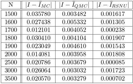
We give the results for the case when M = 5. The following table contains the value of N and the absolute values of the errors|I−I¯M C|,|I−I¯QM C|,|I−I¯RSN U|.
[image:14.595.193.422.456.601.2]N |I−I¯M C| |I−I¯QM C| |I−I¯RSN U| 1500 0.035780 0.003482 0.001617 1600 0.027438 0.005332 0.001305 1700 0.012101 0.004052 0.000238 1800 0.030410 0.004104 0.001907 1900 0.023049 0.004610 0.001543 2000 0.014081 0.003958 0.001808 2500 0.020786 0.003679 0.000085 3000 0.026064 0.003032 0.001723 3500 0.020570 0.003279 0.000702
The numerical results, presented in Table 1, indicate that our RSNU estimate converges faster than the MC and QMC estimates. The error in our combined method is smaller than the error in MC method by approximately a factor of 10. The error in our method gives approximately a factor of 3 improvement over the error in QMC method.
5. Application to finance: Evaluation of Asian Options
In this section, we apply our combined method to evaluate the so-called (discrete sampled) Asian option, driven by the asset dynamics S(t), as defined in (12). The general framework remains the same as in the previous section, only the payoff function is changed. The payoff of an Asian call option is defined by
CT(S) = 1
s
s X
i=1
S(ti)−K
+= max n1
s
s X
i=1
S(ti)−K,0o, (32)
with 0 =t0< t1 < t2 < . . . < ts=T. The constant K≥0 is called the strike price. Thus, we get the following integration problem:
I = Z
Rs S(0)
s
s X
i=1
ePij=1x(j)−K
+
| {z }
A(x)
dH(x) = Z
Rs
A(x)dH(x), (33)
where H(x) = Qsi=1Hi(x(i)), ∀x = (x(1), . . . , x(s)) ∈ Rs, and Hi(x(i)) denotes the distribution function of the so-called log-returns induced by Z(t1), with the corre-sponding density function hi(x(i)). These log increments are independent and NIG distributed, having the common density function defined in (19).
In a similar way to the previous section, we transform the integral (33) to an integral on [0,1]s. We get the following integration problem on [0,1]s:
I = Z
[0,1]s S(0)
s
s X
i=1
ePij=1Hλ−1(z(j))−K
+
| {z }
f(z)
dG(z) = Z
[0,1]s
f(z)dG(z), (34)
where G: (0,1)s→[0,1], defined by
G(z) = s Y
i=1
is a distribution function on (0,1)s, with independent marginals G
i = Hi◦Hλ−1,
i= 1, . . . , s. The inverse function H−1
λ is defined in (21).
The integral I is an improper integral because the function f has singularities on the right boundary of the interval [0,1]s, i.e., lim
z(i)→1f(z(1), . . . , z(s)) =∞ for
i= 1, . . . , s.
In the following, we compare numerically our combined method, with the MC and QMC methods, in terms of absolute errors.
We suppose that the parameters of the NIG-distributed log-returns under the equivalent martingale measure given by the Esscher transform are the same as in (31). We assume that the initial stock price isS(0) = 100, the strike price isK = 100 and the risk-free annual interest rate isr = 3.75%. We choose the parameter of the double-exponential distribution λ= 95.2271.
The Asian call option is sampled weekly. We also let the option to have maturities of 3 weeks. Hence, our problem is a 3-dimensional integral over the payoff function. In a similar way to the previous section, we compute the estimates ¯IM C, ¯IQM C and ¯IRSN U, given by (26), (27) and (30), respectively.
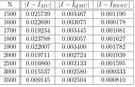
The ”true” price is obtained as the average of 10 MC simulations, with N = 100000. We give the results for the case when M = 7. The following table contains: the value ofN and the absolute values of the errors|I−I¯M C|,|I−I¯QM C|,|I−I¯RSN U|.
[image:16.595.195.424.359.506.2]N |I−I¯M C| |I−I¯QM C| |I−I¯RSN U| 1500 0.025739 0.003467 0.001190 1600 0.022690 0.003075 0.000178 1700 0.019234 0.003445 0.001081 1800 0.023788 0.003057 0.001627 1900 0.022007 0.003400 0.001782 2000 0.019711 0.002724 0.001939 2500 0.016860 0.003133 0.001595 3000 0.015537 0.002580 0.000333 3500 0.009145 0.002504 0.000810 Table 2: Asian Call Option: Case s= 3 and M = 7.
References
[1] O.E. Barndorff-Nielsen, Processes of normal invers Gaussian type, Finance and Stochastic, 2 (1998), 41-68.
[2] P.P. Boyle, Options: A Monte Carlo Approach, J. Financial Economics, 4 (1977), 323-338.
[3] P. Chelson, Quasi-Random Techniques for Monte Carlo Methods, Ph.D Dis-sertation, The Claremont Graduate School, 1976.
[4] R. Cranley, T.N.L. Patterson, Randomization of number theoretic methods for multiple integration, SIAM J. Numer. Anal., 13 (6), December 1976, 904-914.
[5] I. De´ak, Random Number Generators and Simulation, Akad´emiai Kiad´o, Bu-dapest, 1990.
[6] F. Delbaen, W. Schachermayer,A general version of the fundamental theorem of asset pricing, Math. Ann., 300(3) (1994), 463-520.
[7] E. Eberlein, U. Keller,Hyperbolic distribution in finance, Bernoulli, 1 (1995), 281-299.
[8] P. Glasserman, Monte Carlo Methods in Financial Engineering, Springer-Verlag, New-York, 2003.
[9] M. Gnewuch, A.V. Ro¸sca, On G-Discrepancy and Mixed Monte Carlo and Quasi-Monte Carlo Sequences, Acta Universitatis Apulensis, Mathematics-Informatics, 18 (2009), 97-110.
[10] J. Hartinger, R. Kainhofer, Non-Uniform Low-Discrepancy Sequence Gen-eration and Integration of Singular Integrands, Proceedings of Monte Carlo and Quasi-Monte Carlo Methods 2004 (H. Niederreiter, eds.), Springer-Verlag, Berlin, 2006, 163-180.
[11] E. Hlawka,Gleichverteilung und Simulation, ¨Osterreich. Akad. Wiss. Math.-Natur. Kl. Sitzungsber. II, 206 (1997), 183-216.
[12] E. Hlawka, R. M¨uck, A transformation of equidistributed sequences, Appli-cations of number theory to numerical analysis, Academic Press, New-York, 1972, 371-388.
[13] E. Hlawka, R. M¨uck,Uber Eine Transformation von gleichverteilten Folgen¨ , II, Computing, 9 (1972), 127-138.
[14] C. Joy, P.P. Boyle, K.S. Tan, Quasi-Monte Carlo Methods in Numerical Finance, Management Science, 42 (1996), no. 6, 926-938.
[15] R. Kainhofer,Quasi-Monte Carlo Algorithms with Applications in Numerical Analysis and Finance, Ph. D. Dissertation, Graz, April 2003.
[17] S. Ninomiya, S. Tezuka,Toward real-time pricing of complex financial deriva-tives, Applied Mathematical Finance, 3 (1996), 1-20.
[18] H. Niederreiter, Random number generation and Quasi-Monte Carlo meth-ods, Society for Industrial and Applied Mathematics, Philadelphia, 1992.
[19] G. ¨Okten,A Probabilistic Result on the Discrepancy of a Hybrid-Monte Carlo Sequence and Applications, Monte Carlo Methods and Applications, 2 (1996), no. 4, 255-270.
[20] G. ¨Okten,Error Estimation for Quasi-Monte Carlo Methods, In Monte Carlo and Quasi-Monte Carlo Methods 1996 (H. Niederreiter et al., eds.), Lecture Notes in Statistics, Vol. 127, Springer-Verlag, New York, 1998, 353-368.
[21] G. ¨Okten, Error Reduction Techniques in Quasi-Monte Carlo Integration, Math. Comput. Modelling, 30 (1999), no 7-8, 61-69.
[22] G. ¨Okten, B. Tuffin, V. Burago, A central limit theorem and improved er-ror bounds for a hybrid-Monte Carlo sequence with applications in computational finance, Journal of Complexity, 22 (2006), no. 4, 435-458.
[23] A.B. Owen,Randomly permuted (t,m,s)-nets and (t,s)-sequences, In Monte Carlo and Quasi-Monte Carlo Methods in Scientific Computing (Harald Niederreiter et al., eds.), Lecture Notes in Statistics, Vol. 106, Springer, New York, 1995, 299-317. [24] A.B. Owen, Monte Carlo Variance of Scrambled Net Quadrature, SIAM Journal of Numerical Analysis, 34 (1997), 1884-1910.
[25] G. Pag`es, Y.J. Xiao, Sequences with low discrepancy and pseudo-random numbers: theoretical results and numerical tests, J. Statist. Comput. Simulat., 56 (1997), no. 2, 163-188.
[26] K. Prause,The Generalized Hyperbolic Model: Estimation, Financial Deriva-tives and Risk Measures, Ph.D. Dissertation, Albert-Ludwigs-Universitat, Freiburg, 1999.
[27] S. Raible, L´evy Processes in Finance: Theory, Numerics and Empirical Facts, Ph.D. Dissertation, Albert-Ludwigs-Universitat, Freiburg, 2000.
[28] A.V. Ro¸sca, A Mixed Monte Carlo and Quasi-Monte Carlo Sequence for Multidimensional Integral Estimation, Acta Universitatis Apulensis, Mathematics-Informatics, 14 (2007), 141-160.
[29] A.V. Ro¸sca, A Mixed Monte Carlo and Quasi-Monte Carlo Method with Applications to Mathematical Finance, Studia Univ. Babe¸s-Bolyai, Mathematica, 53 (2008), no. 4, 57-76.
[30] N. Ro¸sca,Generation of Non-Uniform Low-Discrepancy Sequences in Quasi-Monte Carlo Integration(in dimension one), Studia Univ. Babe¸s-Bolyai, Mathemat-ica, 50 (2005), no. 2, 77-90.
207-219.
[32] N. Ro¸sca, A Combined Monte Carlo and Quasi-Monte Carlo Method for Estimating Multidimensional Integrals, Studia Univ. Babe¸s-Bolyai, Mathematica, 52 (2007), no. 1, 125-140.
[33] N.C. Ro¸sca,Monte Carlo and Quasi-Monte Carlo Methods with Applications, Cluj University Press, Cluj-Napoca, 2009.
[34] T.H. Rydberg, The normal inverse Gaussian L´evy process: simulation and approximation, Comm. Statist. Stochastic Models, 13 (1997), no. 4, 887-910.
[35] J.E.H. Shaw,A quasirandom approach to integration in Bayesian statistics, Ann. Statist., 16 (1988), 895-914.
[36] J. Spanier, Quasi-Monte Carlo Methods for Particle Transport Problems, Proc. Conf. on Monte Carlo Methods in Scientific Computing, Univ. Las Vegas, 1994.
Natalia C. Ro¸sca Babe¸s-Bolyai University
Faculty of Mathematics and Computer Science