Full Terms & Conditions of access and use can be found at
http://www.tandfonline.com/action/journalInformation?journalCode=ubes20
Download by: [Universitas Maritim Raja Ali Haji] Date: 12 January 2016, At: 00:34
Journal of Business & Economic Statistics
ISSN: 0735-0015 (Print) 1537-2707 (Online) Journal homepage: http://www.tandfonline.com/loi/ubes20
A Pure-Jump Transaction-Level Price Model
Yielding Cointegration
Clifford M. Hurvich & Yi Wang
To cite this article: Clifford M. Hurvich & Yi Wang (2010) A Pure-Jump Transaction-Level Price
Model Yielding Cointegration, Journal of Business & Economic Statistics, 28:4, 539-558, DOI: 10.1198/jbes.2009.07116
To link to this article: http://dx.doi.org/10.1198/jbes.2009.07116
Published online: 01 Jan 2012.
Submit your article to this journal
Article views: 73
A Pure-Jump Transaction-Level Price
Model Yielding Cointegration
Clifford M. H
URVICHand Yi W
ANGStern School of Business, New York University, New York, NY 10012 (churvich@stern.nyu.edu;ywang2@stern.nyu.edu)
We propose a new transaction-level bivariate log-price model that yields fractional or standard cointegra-tion. The model provides a link between market microstructure and lower-frequency observations. The two ingredients of our model are a long-memory stochastic duration process for the waiting times,{τk},
between trades and a pair of stationary noise processes, ({ek}and{ηk}), which determine the jump sizes
in the pure-jump log-price process. Our model includes feedback between the disturbances of the two log-price series at the transaction level, which induces standard or fractional cointegration for any fixed sampling intervalt. We prove that the cointegrating parameter can be consistently estimated by the ordinary least squares estimator, and we obtain a lower bound on the rate of convergence. We propose transaction-level method-of-moments estimators of the other parameters in our model and discuss the consistency of these estimators.
KEY WORDS: Information share; Long-memory stochastic duration; Tick time.
1. INTRODUCTION
We propose a transaction-level, pure-jump model for a bi-variate price series in which the intertrade durations are sto-chastic and enter into the model in a fully endogenous way. The model is flexible and able to capture a variety of styl-ized facts, including standard or fractional cointegration, per-sistence in durations, volatility clustering, leverage (i.e., a neg-ative correlation between current returns and future volatility), and nonsynchronous trading effects. In our model, all of these features observed at equally spaced time intervals are derived from transaction-level properties. Thus the model provides a link between market microstructure and lower-frequency obser-vations. This article focuses on the cointegration aspects of the model, presenting theoretical, simulation, and empirical analy-ses.
Cointegration is a well-known phenomenon that has received considerable attention in economics and econometrics. Under both standard and fractional cointegration, there is a contempo-raneous linear combination of two or more time series that is less persistent than the individual series. Under standard coin-tegration, the memory parameter is reduced from 1 to 0, while under fractional cointegration, the level of reduction need not be an integer. Indeed, in the seminal article of Engle and Granger
(1987), both standard and fractional cointegration were allowed
for, although the literature has since developed separately for the two cases. Important contributions to the representation, es-timation, and testing of standard cointegration models include
those of Stock and Watson (1988), Johansen (1988,1991), and
Phillips (1991a). Literature addressing the corresponding
prob-lems in fractional cointegration includes works by Dueker and
Startz (1998), Marinucci and Robinson (2001), Robinson and
Marinucci (2001), Robinson and Yajima (2002), Robinson and
Hualde (2003), Velasco (2003), Velasco and Marmol (2004),
and Chen and Hurvich (2003a,2003b,2006).
A limitation of most existing models for cointegration is that
they are based on a particular fixed sampling interval,t(e.g.,
1 day, 1 month) and thus do not reflect the dynamics at all
lev-els of aggregation. Indeed, Engle and Granger (1987) assumed
a fixed sampling interval. It is also possible to build models
for cointegration using diffusion-type continuous-time models, such as ordinary or fractional Brownian motion (see Phillips
1991b; Comte and Renault1996,1998; Comte1998), but such models would fail to capture the pure-jump nature of observed asset-price processes.
In this article we propose a pure-jump model for a bivari-ate log-price series such that any discretization of the process
to an equally spaced sampling grid with sampling intervalt
produces fractional or standard cointegration; that is, there ex-ists a contemporaneous linear combination of the two log-price series that has a smaller memory parameter than the two indi-vidual series. A key ingredient in our model is a microstructure
noise contribution,{ηk}, to the log prices. In theweak fractional
cointegrationcase, this noise series is assumed to have memory
parameter dη∈(−12,0)in the strong fractional cointegration
casedη∈(−1,−12), while in thestandard cointegrationcase,
dη= −1. In all three cases, the reduction of the memory
para-meter is−dη. Due to the presence of the microstructure noise
term, the discretized log-price series are not martingales, and the corresponding return series are not linear in an iid sequence, a martingale-difference sequence, or a strong-mixing sequence. This is in sharp contrast to existing discrete-time models for cointegration, most of which assume at least that the series has a linear representation with respect to a strong-mixing sequence. The discretely sampled returns (i.e., the increments in the log-price series) in our model are not martingale differences, because of the microstructure noise term. Instead, for small
values oft they may exhibit noticeable autocorrelations, as
also seen in actual returns over short time intervals. Neverthe-less, the returns behave asymptotically like Martingale
differ-ences as the sampling intervaltis increased, in the sense that
the lag-kautocorrelation tends to 0 asttends to ∞for any
fixedk. Again, this is consistent with the near-uncorrelatedness
observed in actual returns measured over long time intervals.
© 2010American Statistical Association Journal of Business & Economic Statistics
October 2010, Vol. 28, No. 4 DOI:10.1198/jbes.2009.07116
539
The memory parameter of the log prices in our model is 1, in
the sense that the variance of the log price increases linearly int
asymptotically ast→ ∞. In contrast, the memory parameter of
the appropriate contemporaneous linear combination of the two
log-price series is reduced to(1+dη) <1, thereby establishing
the existence of cointegration in our model.
To derive the results described herein, we make use of the general theory of point processes, and also rely heavily on the
theory developed by Deo et al. (2009) for the counting process
N(t)induced by a long-memory duration process. In Section2
we present our pure-jump model for the bivariate log-price se-ries. Because the two series need not have all of their transac-tions at the same time points (due to nonsynchronous trading), it is not possible to induce cointegration in the traditional way, that is, by directly imposing in clock time (calendar time) an additive common component for the two series with a mem-ory parameter equal to 1. Instead, the common component is induced indirectly, and incompletely, by means of a feedback mechanism in transaction time between current log-price dis-turbances of one asset and previous log-price disdis-turbances of the other asset. This feedback mechanism also induces certain end-effect terms, which we explicitly display and handle in our theoretical derivations using the theory of point processes.
The article is organized as follows. In Section2we provide
economic justification for the model, as well as a transaction-level definition of the information share of a market. We also present some preliminary data analysis results that affirm the potential usefulness of certain flexibilities in the model. In
Sec-tion3we define conditions on the microstructure noise process
for both fractional and standard cointegration. These conditions are satisfied by various standard time series models. In
Sec-tion4we present the properties of the log-price series implied
by our model. In particular, we show that the log price behaves
asymptotically like a martingale astis increased, and that the
discretely sampled returns behave asymptotically like
Martin-gale differences as the sampling intervaltis increased. In
Sec-tion5we establish that our model has cointegration, by
show-ing that the cointegratshow-ing error has memory parameter(1+dη).
We present separate theorems for the weak and strong frac-tional cointegration and standard cointegration cases. In
Sec-tion 6we show that the ordinary least squares (OLS)
estima-tor of the cointegrating parameterθis consistent, and obtain a
lower bound on its rate of convergence. In Section 7we
pro-pose an alternative cointegrating parameter estimator based on
the tick-level price series. In Section8, we propose a
method-of-moments estimator for the tick-level model parameters
(ex-cept the cointegrating parameterθ). The method is based on the
observed tick-level returns. In Section9we propose a
specifica-tion test for the transacspecifica-tion-level price model, and in Secspecifica-tion10
we present simulation results on the OLS estimator of θ, the
tick-level cointegrating parameter estimator θ˜, the
method-of-moments estimator, and the proposed specification test. In
Sec-tion11we present a data analysis of buy and sell prices of a
sin-gle stock (Tiffany; TIF), providing evidence of strong fractional cointegration. The cointegrating parameter is estimated by both OLS regression and the alternative tick-level method proposed
in Section7. The proposed specification test is implemented on
the data. Interesting results are observed that are consistent with the existing literature about price discovery process in a market-dealer market. We then consider the information content of buy
trades versus sell trades in different market environments. In
Section12we provide some concluding remarks and discuss
possible further generalizations of our model and related future
work. We provide proofs in theAppendix.
2. A PURE–JUMP MODEL FOR LOG PRICES
Before describing our model, we provide some background on transaction-level modeling. Currently, a wealth of tran-saction-level price data is available, and for such data, the (ob-served) price remains constant between transactions. If there is a diffusion component underlying the price, it is not directly observable. Thus pure-jump models for prices provide a poten-tially appealing alternative to diffusion-type models. The
com-pound Poisson process proposed by Press (1967) is a pure-jump
model for the logarithmic price series under which innovations to the log price are iid, and these innovations are introduced at random time points, determined by a Poisson process. The
model was generalized by Oomen (2006), who introduced an
additional innovation term to capture market microstructure. An informative and directly observable quantity in
tran-saction-level data is the duration{τk}between transactions. In a
seminal article focusing on durations and, to some extent, on the
induced price process, Engle and Russell (1998) documented
a key empirical fact that durations are strongly autocorrelated, quite unlike the iid exponential duration process implied by a Poisson transaction process, and they proposed the autoregres-sive conditional duration (ACD) model, which is closely related to the generalized autoregressive conditional heteroscedasticity
model of Bollerslev (1986). Deo, Hsieh, and Hurvich (2006)
presented empirical evidence that durations, as well as transac-tion counts, squared returns, and realized volatility, have long memory, and introduced the long-memory stochastic duration (LMSD) model, which is closely related to the long-memory
stochastic volatility model of Breidt, Crato, and de Lima (1998)
and Harvey (1998). The LMSD model is τk =ehkǫk, where
{hk}is a Gaussian long-memory series with memory
parame-terdτ∈(0,12), the{ǫk}are iid positive random variables with
mean 1, and{hk}and{ǫk}are mutually independent.
Deo et al. (2009) demonstrated that long memory in
dura-tions propagates to long memory in the counting processN(t),
whereN(t)counts the number of transactions in the time
in-terval(0,t]. In particular, if the durations are generated by an
LMSD model with memory parameterdτ∈(0,12), thenN(t)is
long-range count–dependent with the same memory parameter,
in the sense that varN(t)∼Ct2dτ+1ast→ ∞. This long-range
count dependence then propagates to the realized volatility, as
studied by Deo et al. (2009).
We now describe the tick-time return interactions that yield cointegration in our model. Suppose that there are two assets, 1 and 2, and that each log price is affected by two types of distur-bances when a transaction occurs. These disturdistur-bances are the value shocks,{ei,k}, and the microstructure noise,{ηi,k}, for
as-seti=1,2. The subscripti,kpertains to thekth transaction of
asseti. The value shocks are iid and represent permanent
con-tributions to the intrinsic log value of the assets, which in the absence of feedback effects is a martingale with respect to full information, both public and private (see Amihud and
Mendel-son1987; Glosten1987). The microstructure shocks represent
Figure 1. Changes in log prices. The online version of this figure is in color.
the remaining contributions to the observed log prices, along similar lines as the noise process considered by Amihud and
Mendelson (1987), reflecting transitory price fluctuations due
to, for example, liquidity impact of orders. We assume that the
mth tick-time return of asset 1 incorporates not only its own
current disturbancese1,mandη1,m, but also weighted versions
of all intervening disturbances of asset 2 that were originally
introduced between the(m−1)th andmth transactions of
as-set 1. The weight for the value shocks, denoted byθ, may differ
from the weight for the microstructure noise, denoted byg21
(the impact from asset 2 to asset 1). We similarly define themth
tick-time return of asset 2, but the weight for the value shocks
from asset 1 to asset 2 is(1/θ ), and the corresponding weight
for the microstructure noise is denoted byg12. The choice of
the second impact coefficient (1/θ ) is necessary for the two
log-price series to be cointegrated. In general, if the two series are not cointegrated, then this constraint is not required.
Figure1illustrates the mechanism by which tick-time returns
are generated in our model. All disturbances originating from asset 1 are shown in blue, and all disturbances originating from asset 2 are shown in red. When the first transaction of asset 1
occurs, a value shocke1,1and a microstructure disturbanceη1,1
are introduced. The first transaction of asset 2 follows in clock time, and because the first transaction of asset 1 occurred
be-fore it, the return for this transaction is(e2,1+η2,1+1θe1,1+
g12η1,1), that is, the sum of the first value shock of asset 2,
e2,1, the first microstructure disturbance of asset 2,η2,1, and a feedback term from the first transaction of asset 1 whose
distur-bances aree1,1andη1,1, weighted by the corresponding
feed-back impact coefficientsθ1andg12. In the figure, both log-price
processes evolve until timet. Notice that the third return of
as-set 1 contains no feedback term from asas-set 2, because there is no intervening transaction of asset 2. The second return of
as-set 2 includes its own current disturbances (e2,2,η2,2) as well as
six weighted disturbances (e1,2,e1,3,e1,4,η1,2,η1,3, andη1,4)
from asset 1, because there are three intervening transactions of asset 1.
At a given clock timet, most of the disturbances of asset 1 are
incorporated into the log price of asset 2 and vice-versa. There
is anend effect, however. The problem is readily seen in the
figure: because the fifth transaction of asset 1 occurred after the
last transaction of asset 2 before timet, the most recent asset 1
disturbancese1,5andη1,5are not incorporated in the log price
of asset 2 at timet. Eventually, at the next transaction of asset 2,
which will occur after time t, these two disturbances will be
incorporated. But this end effect may be present at any given
timet. We handle this end effect explicitly in all derivations in
this article.
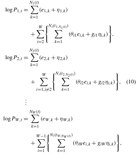
Our model for the log prices for all nonnegative realtis then
given by
logP1,t= N1(t)
k=1
(e1,k+η1,k)+
N2(t1,N1(t))
k=1
(θe2,k+g21η2,k),
(1)
logP2,t= N2(t)
k=1
(e2,k+η2,k)+
N1(t2,N2(t))
k=1
1
θe1,k+g12η1,k
,
whereti,kis the clock time for thekth transaction of assetiand
Ni(t) (i=1,2)are counting processes that count the total
num-ber of transactions of assetiup to timet. Later we impose
spe-cific conditions on{ei,k},{ηi,k}, andNi(t). Note that (1) implies
that logP1,0=logP2,0=0, the same standardization used by
Stock and Watson (1988) and others. The quantityN2(t1,N1(t))
represents the total number of transactions of asset 2 occurring
up to the time (t1,N1(t)) of the most recent transaction of asset 1.
An analogous interpretation holds for the quantityN1(t2,N2(t)).
To exhibit the various components of our model, we rewrite (1) as
logP1,t= N1(t)
k=1
e1,k+ N2(t)
k=1
θe2,k
common component
+ N
1(t)
k=1
η1,k+ N2(t)
k=1
g21η2,k
microstructure component
−
N2(t)
k=N2(t1,N1(t))+1
(θe2,k+g21η2,k)
end effect
,
(2)
logP2,t= N
1(t)
k=1 1
θe1,k+ N2(t)
k=1
e2,k
common component
+ N1(t)
k=1
g12η1,k+ N2(t)
k=1
η2,k
microstructure component
−
N1(t)
k=N1(t2,N2(t))+1
1
θe1,k+g12η1,k
end effect
.
The common component is a martingale and thus isI(1). We
show that the microstructure components areI(1+dη), so these
components are less persistent than the common component. The end-effect terms are random sums over time periods that
areOp(1)ast→ ∞[see (A.10) to (A.12)] and thus are
negli-gible compared with all other terms. Because both logP1,tand
logP2,t are I(1)(see Theorem1) and the linear combination
logP1,t−θlogP2,tisI(1+dη)as defined in Section3, the
log-price series are cointegrated (see Theorems3,4, and5).
Frijns and Schotman (2006) considered a mechanism for
generating quotes in tick time that is similar to the
mecha-nism shown in Figure1; however, they condition on durations,
whereas we endogenize them in our model (1). Furthermore,
their model implies standard cointegration, with a cointegrating parameter known to be 1 and a single value shock component.
Throughout the article, unless noted otherwise, we make the following assumptions for our theoretical results. The duration
processes{τi,k}of asseti(i=1,2), are assumed to have long
memory with memory parameters dτ1,dτ2 ∈(0,
1
2), to reflect the empirically observed persistence in durations and the
re-sulting realized volatility. Specifically, the{τi,k}are assumed to
satisfy the assumptions in theorem 1 of Deo et al. (2009), which
are very general and would allow, for example, the LMSD
model of Deo, Hsieh, and Hurvich (2006).
We assume that the {ei,k} are mutually independent iid
processes with mean 0 and variance σi2,e (i=1,2). We also
assume that the{ηi,k}are mutually independent, with mean 0
and memory parameterdηi. For notational convenience, we set
dη1=dη2=dηin our theoretical results. All theorems will
con-tinue to hold, however, whendη1anddη2are distinct, simply by
replacingdη withdη∗=max(dη1,dη2). For Theorem6, which
establishes the consistency of the OLS estimator ofθ, we
fur-ther assume{ei,k}to be N(0, σi2,e).
We assume that{τ1,k}and{τ2,k}are independent of all
dis-turbance series{e1,k},{e2,k},{η1,k}, and{η2,k}, which we
as-sume to be mutually independent. But we do not require that
N1(·) andN2(·)be mutually independent, nor that {τ1,k}and
{τ2,k}be mutually independent. This is in keeping with recent
literature suggesting that feedback occurs between the counting
processes (see, e.g., Nijman, Spierdijk, and Soest2004;
Bow-sher2007; and references therein).
2.1 Economic Justification for the Model
Here we provide some economic rationale for the
transaction-level return interactions leading to model (1). This supplements
our earlier discussion around Figure1on the formal mechanism
for price formation. After a brief data analysis affirming the po-tential usefulness of certain flexibilities of the model, we com-pare and contrast the model with a clock-time model proposed
by Hasbrouck (1995), and then propose a transaction-level
gen-eralization of Hasbrouck’s definition of the information share of a market.
The model (1) is potentially economically appropriate for
pairs of measured prices that are both affected by the same information shocks (i.e., value shocks), possibly in different ways. Examples include buy prices and sell prices of a sin-gle stock, prices of two classified stocks (with different voting rights) from a given company, prices of two different stocks within the same industry, stock and option prices of a given company, option prices on a given stock with different degrees of maturity or moneyness, corporate bond prices at different maturities for a given company, and Treasury bond prices at different maturities.
The fundamental (value) prices at timetare an accumulation
of information shocks. If we ignore the end effects, then these fundamental prices may be thought of as the common
compo-nents in (2). More precisely, the fundamental prices may be
ob-tained by setting the microstructure shocks in (1) to 0. For
def-initeness, consider the example of buy prices (asset 1) and sell prices (asset 2) of a single stock. Information shocks may be generated on either the buy side or the sell side. According to the model, each buy transaction generates its own information shock, as does each sell transaction. Furthermore, these shocks spill over from the side of the market in which they originated to the other side. Clearly, shocks originating from the sell side of the market cannot be impounded into the buy price until there is a transaction on the buy side. Similarly, in the absence of in-formation arrivals (transactions) on the sell side, any string of intervening information shocks from the buy side will render the most recent sell price stale, until the intervening buy-side shocks are actually impounded into the sell-side price at the next sell transaction.
Shocks spilling over from the buy side to the sell side are
weighted by 1/θ, while those spilling from the sell side to the
buy side are weighted byθ. Whenθ=1, shocks spill over from
one side to the other in an identical way, and there is just a sin-gle fundamental price, shared by both the buy side and sell side.
In general, as can be seen from (1), the fundamental (log) price
for the buy side is an accumulation of information shocks from both the buy side and the sell side, with the sell-side shocks
weighted byθ. Ignoring end effects, as can be seen from (2),
the common component on the buy side is proportional to the common component on the sell side, and the constant of
pro-portionality isθ.
Analogous interactions take place on the microstructure shocks, such that a microstructure shock originating on the buy
side spills over to the sell side with weightg12, and the
oppo-site spillover occurs with weight g21. Even in the absence of
spillover of the microstructure shocks (g12=g21=0), the
dif-ference between the buy price andθtimes the sell price is
(ex-cept for end effects) an accumulation of microstructure shocks. It seems to be in accordance with the economic connotation of the term “microstructure” that the microstructure shocks be transitory, that is, the aggregate of microstructure shocks be
stochastically of smaller order than the aggregate of
funda-mental shocks, as t→ ∞. This will occur if and only if the
microstructure shocks have a smaller memory parameter than
the fundamental shocks (dη <0), as we assume.
Cointegra-tion arises as a consequence of the spillover of the fundamental
shocks, together with the assumptiondη<0. The spillover of
the fundamental shocks induces the common component, while
the assumptiondη<0 ensures that the cointegrating error
aris-ing from the microstructure is less persistent than the common component.
Two questions that might be raised in the context of model
(1) are whether there are situations in which the two prices are
affected by information in different ways, so that the cointe-grating parameter is not equal to 1, and whether it is helpful in practice to allow for fractional cointegration as opposed to standard cointegration. To address these questions, we briefly present some results of a preliminary data analysis. We consid-ered clock-time option best-available-bid prices and underlying best-available-bid prices for IBM on the NYSE at 390 1-minute intervals from 9:30 a.m. to 4 p.m. on May 31, 2007. We origi-nally analyzed 74 different options, but removed 5 from consid-eration because they had either at least one zero bid price during the day or a constant bid price throughout the day. For the re-maining 69 options, we regressed the log stock bid price on the log option bid price, and constructed a semiparametric GPH
es-timator (Geweke and Porter-Hudak1983) of the memory
pa-rameter of the residuals. The least squares regression slopes
ranged from−0.21 to 0.39, with a mean of 0.04 and a
stan-dard deviation of 0.13. This suggests that information affected
the two prices in different ways for all 69 options. For the GPH
estimators, we used 3900.5for the number of frequencies; this
resulted in an approximate standard error for the GPH estimator of 0.19. The GPH estimator for the log stock bid price was 1.02. The GPH estimators for the residuals ranged from 0.05 to 1.14, with a mean of 0.55 and a standard deviation of 0.28. Of the
69 sets of residuals, 62 yielded a GPH estimator<1, with 54
<0.75, 42<0.6, and 18 between 0.4 and 0.6. These results
sug-gest the presence of cointegration in most cases, and also imply that the cointegration in some of these cases may be fractional instead of standard.
It is instructive to compare and contrast our model (1) with
the clock-time model of Hasbrouck (1995), in which a single
security is traded on several markets and different market prices share an identical random-walk component. To facilitate
com-parisons with the bivariate model (1), suppose that there are two
markets. Then for all nonnegative integersj, the clock-time log
stock prices at timejon the two different markets, are given by
Hasbrouck’s model as
logP1,j=logP1,0+
j
s=1
(ψ1e˜1,s+ψ2e˜2,s)+v1,j,
(3)
logP2,j=logP2,0+
j
s=1
(ψ1e˜1,s+ψ2e˜2,s)+v2,j,
where logP1,0and logP2,0are constants,(˜e1,s,e˜2,s)′is a
mean-0 vector of serially uncorrelated disturbances with covariance
matrix , ψ =(ψ1, ψ2) are the weights for e˜1,s,e˜2,s, and
{(v1,j,v2,j)′}is a mean-0 stationary bivariate time series. The
quantity e˜i,s (i=1,2) may be considered the fundamental
shock originating from the ith market. Hasbrouck (1995)
es-timated the model on data using a 1-second sampling interval.
Both models (1) and (3) induce a common component, as
well as cointegration. Both contain spillover of the fundamental
shocks from one market to the other. In model (3) the spillover
is the same in both directions, so the common components are identical and the cointegrating parameter is 1. In contrast, in
model (1) the cointegrating parameter need not be equal to 1.
In model (3) the cointegrating error isI(0), while in model (1)
the cointegrating error is allowed to beI(1+dη)for anydηwith
−1≤dη<0.
In model (3) the contemporaneous correlation between the
fundamental shocks originating from the two markets is
al-lowed to be nonzero, (i.e., is allowed to be nondiagonal),
whereas in model (1) the two fundamental shock series are
as-sumed to be independent. Note, however, that in the
transaction-level model (1), the kth transactions of the two assets will
(al-most surely) occur at different clock times, so any correlation
between the two fundamental shockse1,kande2,kwould not be
contemporaneous in clock time. This provides a motivation for
our assumption that{e1,k}and{e2,k}are mutually independent.
An economic motivation for this assumption stems from the
following remarks of Hasbrouck (1995, p. 1183): “In practice,
market prices usually change sequentially: a new price is posted in one market, and then the other markets respond. If the obser-vation interval is so long that the sequencing cannot be deter-mined, however, the initial change and the response will appear to be contemporaneous. Therefore, one obvious way of mini-mizing the correlation is to shorten the interval of observation.”
Because model (1) is defined in continuous time, the interval
of observation is effectively zero, so at least under the idealized assumptions that there are no truly simultaneous transactions on the two markets and that the time stamps for the transac-tions are exact, the assumption of mutual independence would be economically reasonable.
In the remainder of this section, we discuss the information
share, originally defined by Hasbrouck (1995) to measure how
market information that drives stock prices is distributed across
different exchanges. Hasbrouck (1995) defined the information
share of marketibased on model (3) asSi=(ψi2 ii)/(ψ ψ′),
which is the proportional contribution from marketito the total
fundamental innovation variance. Only the random-walk com-ponent is used in constructing the information share, because
this is the only permanent component. As Hasbrouck (1995)
discussed, because may not be diagonal, only a bound for
the information share can be estimated. Here we propose a transaction-level generalization of the concept of information
share based on model (1), which is directly estimable because
of our assumption of mutual independence of the transaction-level fundamental disturbance series. The information share
proposed by Hasbrouck (1995) measures how the price
discov-ery of one security is fulfilled across difference exchanges. In contrast, our information share instead measures how the price-driving information of a security is distributed between buy ver-sus sell trades in a market. The ideas are similar. Indeed, as
Has-brouck (1995) noted, his model can be extended to model bid
and ask price dynamics. Nevertheless, as discussed earlier, our model ultimately is a tick-level model that differs from existing
clock-time models, including that of Hasbrouck (1995).
For model (1), we define the information share as follows.
For a given clock-time sampling interval t, the information
share of assetiis given by
S1,C=
var(N1(jt)
k=N1((j−1)t)+1e1,k)
var(N1(jt)
k=N1((j−1)t)+1e1,k+θ
N2(jt)
k=N2((j−1)t)+1e2,k)
= λ1σ
2 1,e
λ1σ1,2e+θ2λ2σ2,2e
, (4)
S2,C=
θ2λ2σ2,2e
λ1σ1,2e+θ2λ2σ2,2e
,
whereλiis the intensity of the counting processNi(·)(see
Da-ley and Vere-Jones2003) and represents the intensity of trading
(level of market activity) of asseti. The ultimate expressions for
Si,Cdo not depend on the sampling intervalt. Note that only
the common component in (2) is used to evaluate the
informa-tion share, as was done by Hasbrouck (1995). Asλ1/λ2→ ∞,
S1,C approaches 1 and S2,C approaches 0. This is consistent
with general intuition; an actively traded security should reveal more information than a thinly traded one. Indeed, Hasbrouck
(1995) found that for the 30 Dow Jones stocks, the
preponder-ance of the price discovery occurs at the NYSE and the majority of the transactions occur on the NYSE. The information share
Si,Ccan be estimated using the transaction-level method of
mo-ments, as described in Section8. We present estimates ofSi,C
computed from transaction-level data in Section11.
3. CONDITIONS ON THE MICROSTRUCTURE NOISE FOR FRACTIONAL AND STANDARD COINTEGRATION
In this section we consider three types of cointegration: weak fractional, strong fractional, and standard cointegration. We de-scribe the conditions assumed for each of these three cases sep-arately.
The weak fractional cointegration case corresponds todη∈
(−12,0). In this case, we require the following condition, stated
for a generic process{ηk}:
Condition A. Fordη∈(−12,0),{ηk}is a weakly stationary
mean-0 process with memory parameterdηin the sense that the
spectral densityf(λ)satisfies
f(λ)= ˜σ2C∗λ−2dη(1+O(λβ)) asλ→0+
for some β with 0< β ≤2, where σ˜2>0 and C∗=(dη+
1
2)Ŵ(2dη+1)sin((dη+ 1
2)π )/π >0.
ConditionA, which was originally used in a
semiparamet-ric context by Robinson (1995), is very general, specifying
only the behavior of the spectral density in a neighborhood of zero frequency. The condition is satisfied by all parametric long-memory models that we have seen in the literature,
in-cluding the ARFIMA(p,dη,q) model with p≥0, q≥0, and
dη∈(−12,0). In the ARFIMA case,β =2. Condition Aalso
allows the possibility for seasonal long memory, that is, poles
or 0s off(λ)at nonzero frequencies.
The strong fractional cointegration case corresponds todη∈
(−1,−12). For this case, we assume the following:
Condition B. For dη ∈ (−1,−12), ηk =ϕk −ϕk−1, k =
1,2, . . . , whereϕ0=0 and {ϕk}∞k=1 is a mean-0, weakly
sta-tionary long-memory process with memory parameter dϕ =
dη+1∈(0,12)in the sense that its autocovariances satisfy
cov(ϕk, ϕk+j)=Kj2dϕ−1+O(j2dϕ−3), j≥1, (5)
whereK>0.
By theorem 1 of Lieberman and Phillips (2006), any
sta-tionary, invertible ARFIMA(p,dϕ,q)process withdϕ∈(0,12)
has autocovariances satisfying (5), with K = 2f∗(0)Ŵ(1 −
2dϕ)sin(πdϕ), wheref∗(0)is the spectral density of the ARMA
component of the model at zero frequency.
The standard cointegration case corresponds todη= −1. In
this case we assume the following:
Condition C. Ifdη= −1, then{ηk}∞k=1is given byηk=ξk−
ξk−1withξ0=0. The process{ξk}∞k=1is weakly stationary with
mean 0 and autocovariance sequence{cξ,r}∞r=0, where cξ,r =
E(ξk+rξk)with exponential decay and|cξ,r| ≤Aξe−Kξr for all
r≥0, whereAξ andKξ are positive constants.
The assumptions on{ξk}in ConditionCare satisfied by all
stationary invertible ARMA models.
4. LONG–TERM MARTINGALE–TYPE PROPERTIES OF THE LOG PRICES
In this section we present the properties of the log-price
se-ries generated by model (1). Defineλi=1/E0(τi,k), whereE0
denotes expectation under the Palm distribution (see Deo et al.
2009for information on the Palm probability measure), that is,
the distribution under which the{τi,k}(i=1,2)are stationary.
The following two theorems show that the log-price series in
model (1) have asymptotic variances that scale liketast→ ∞,
as would happen for a martingale, and that their discretized dif-ferences are asymptotically uncorrelated as the sampling inter-val increases, as would occur for a martingale difference series.
Theorem 1. For the log-price series in model (1),
var(logPi,t)∼Cit, i=1,2,
ast→ ∞, whereC1=(σ1,2eλ1+θ2σ2,2eλ2)andC2=(σ2,2eλ2+ 1
θ2σ1,2eλ1).
For a given sampling interval (equally spaced clock-time
pe-riod)t, the returns (changes in log price) for assets 1 and 2
corresponding to model (1) are
r1,j=
N1(jt)
k=N1((j−1)t)+1
(e1,k+η1,k)
+
N2(t1,N1(jt))
k=N2(t1,N1((j−1)t))+1
(θe2,k+g21η2,k),
(6)
r2,j=
N2(jt)
k=N2((j−1)t)+1
(e2,k+η2,k)
+
N1(t2,N2(jt))
k=N1(t2,N2((j−1)t))+1
1
θe1,k+g12η1,k
.
Theorem 2. For any fixed integerk>0, the lag-k autocorre-lation of{ri,j}∞j=1,i=1,2,tends to 0 ast→ ∞.
5. PROPERTIES OF THE COINTEGRATING ERROR
Here we show that model (1) implies a cointegrating
rela-tionship between the two series, treating the weak and strong fractional as well as standard cointegration cases separately.
Theorem 3. Under model (1) withdη∈(−12,0), the
mem-ory parameter of the linear combination(logP1,t−θlogP2,t)
is(1+dη)∈(12,1), that is,
var(logP1,t−θlogP2,t)∼Ct2dη+1
ast→ ∞, whereC>0. In this sense, logP1,t and logP2,tare
weakly fractionally cointegrated.
We next investigate the standard cointegration case. It is
im-portant to note that, unlike in Theorem3, where we measure
the strength of cointegration using the asymptotic behavior of
the variance of the cointegrating errors var(logP1,t−θlogP2,t),
we need a different measure here, because logP1,t−θlogP2,t
is stationary and its variance is constant for allt. Instead, we
consider the asymptotic covariance of the cointegrating errors,
cov(logP1,t−θlogP2,t,logP1,t+j−θlogP2,t+j)
asj→ ∞. Here we taketandjto be positive integers; that is,
we sample the log-price series usingt=1, without loss of
generality.
Theorem 4. Under model (1) withdη∈(−1,−12), the
mem-ory parameter of the cointegrating error(logP1,t−θlogP2,t)is
(1+dη)∈(0,12); that is, for any fixedt>0, cov(logP1,t−θlogP2,t,logP1,t+j−θlogP2,t+j)
∼j2(1+dη)−1C1Pr{N1(t) >0} +C2Pr{N2(t) >0}
as j→ ∞, whereC1>0, C2>0. In this sense, logP1,t and
logP2,tare strongly fractionally cointegrated.
We say that a sequence{aj}hasnearly exponential decayif
aj/j−α→0 asj→ ∞for allα >0. We say that a time series
hasshort memoryif its autocovariances have nearly exponential decay.
Theorem 5. Under model (1), withdη= −1, the
cointegrat-ing error(logP1,t−θlogP2,t)has short memory. In this sense,
logP1,tand logP2,tare cointegrated.
6. LEAST SQUARES ESTIMATION OF THE COINTEGRATING PARAMETER
Assume that the log-price series are observed at integer
mul-tiples oft. The proposed model (1) becomes (with a minor
abuse of notation)
logP1,j= N1(jt)
k=1
(e1,k+η1,k)+
N2(t1,N1(jt))
k=1
(θe2,k+g21η2,k),
(7)
logP2,j= N2(jt)
k=1
(e2,k+η2,k)+
N1(t2,N2(jt))
k=1
1
θe1,k+g12η1,k
.
We show that the cointegrating parameterθ can be
consis-tently estimated by OLS regression.
Theorem 6. For the discretely sampled log-price series in (7)
with normally distributed value shocks{e1,k},{e2,k}, the
cointe-grating parameterθcan be consistently estimated byθˆ, the OLS
estimator obtained by regressing {logP1,j}nj=1 on {logP2,j}nj=1
without intercept. For allδ >0, asn→ ∞, we have
Case I: dη∈(−12,0)
n−dη−δ(θˆ−θ )−→p 0,
Case II: dη∈(−1,−12)
n1/2−δ(θˆ−θ )−→p 0,
Case III: dη= −1
n1−δ(θˆ−θ )−→p 0.
In the weak fractional cointegration case,dη∈(−12,0), the
rate of convergence ofθˆimproves asdηdecreases. In the
stan-dard cointegration case where dη= −1, the rate is arbitrarily
close ton. Phillips and Durlauf (1986) and Stock (1987) have
demonstrated then-consistency (super-consistency) of the OLS
estimator of the cointegrating parameter in the standard cointe-gration case for time series in discrete clock time that are linear with respect to a strong-mixing or iid sequence. We are cur-rently unable to derive the asymptotic distribution of the OLS estimator of the cointegrating parameter in the standard coin-tegration case for our model, because we cannot rely on the strong-mixing condition on returns. This condition would not be expected to hold in the case of LMSD durations, because these are not strong mixing in tick time. In the strong
frac-tional cointegration case dη∈(−1,−12), even though we
es-tablished a rate of n1/2−δ, simulations in Section 10 indicate
that the actual rate is faster, at n−dη−δ, in keeping with the
rates obtained in the weak fractional and standard cointegration cases.
7. A TICK–LEVEL COINTEGRATING PARAMETER ESTIMATOR
In this section we propose a transaction-level estimator,θ˜, for
the cointegrating parameterθ. It may be argued that the OLS
estimatorθˆdiscussed in Section6is not optimal, because it is
constructed based on discretized log-prices and thus uses only
partial information. Here we propose a tick-level estimator,θ˜,
that uses the full tick-level price series, logP1,t, logP2,tfort∈
[0,T].
Specifically, letN(T)=N1(T)+N2(T)be the pooled
count-ing process of transactions for both asset 1 and asset 2 in the time interval(0,T], and let{tk⋆}Nk=(T1)denote the transaction times for the pooled process. The proposed estimator is
˜
θ= T
0 logP1,t·logP2,tdt
T
0 logP 2 2,tdt
=
N(T)−1
j=1
logP1,N1(tj⋆)·logP2,N2(tj⋆)
·(t⋆j+1−tj⋆)
+logP1,N1(T)·logP2,N2(T)
·T−t⋆N(T)
N2(T)−1
j=1
logP22,j·τ2,j+1
+logP22,N
2(T)·
T−t2,N2(T)
, (8)
where the numerator is a summation over all transactions, adding up the product of the most recent log prices of as-sets 1 and 2 weighted by the corresponding duration for the
pooled process. The denominator of θ˜ has the same structure,
except that the product is now of asset 2 log prices with them-selves.
We do not derive asymptotic properties of the estimator θ˜.
Nevertheless, the simulation study presented in Section10
indi-cates that the tick-level estimatorθ˜may outperform the OLS
es-timatorθˆ, having smaller bias, variance, and root mean squared
error (RMSE), particularly if the sampling intervaltforθˆis
large.
8. METHOD–OF–MOMENTS PARAMETER ESTIMATION
In earlier work (Hurvich and Wang 2009), we proposed a
transaction-level parameter estimation procedure for model (1)
using the method of moments, based on logP1,t, logP2,t for
t∈ [0,T]. To conserve space, we omit the complete details
on how we constructed the method-of-moments estimators here. We make specific assumptions for the sake of definite-ness, although most of these assumptions could be relaxed.
Specifically, in constructing our estimates of , we assume
Gaussian white noise for the value shocks and a Gaussian
ARFIMA(1,dη,0)process for the microstructure noise when
dη∈(−12,0), and also assume that the microstructure noise is
the difference of a Gaussian ARFIMA(1,dη +1,0) process
with the initial value set to 0 when dη ∈(−1,−12). In the
standard cointegration case dη= −1, we assume that the
mi-crostructure noise is the difference of a Gaussian AR(1)process
with initial value set to 0. We denote the autoregressive para-meters (lag-1 autocorrelations) of the two microstructure noise
series byα1andα2. The method-of-moments estimator,ˆ =
(σˆ1,2e,σˆ2,2e,σˆ1,η2 ,σˆ2,η2 ,gˆ21,gˆ12,dˆη1,dˆη2,αˆ1,αˆ2), is obtained as
the solution to the following system of equations, based on certain specific observed sequences of assets 1 and 2 transac-tions:
var(second transaction of Sequence 1 1)= ˆσ1,2e+ ˆσ1,η2 ,
var(second transaction of Sequence 2 2)= ˆσ2,2e+ ˆσ2,η2 ,
cov(first and second transactions of Sequence 1 1)
= ˆσ1,η2 ρˆ1,1,
cov(first and second transactions of Sequence 2 2)
= ˆσ2,η2 ρˆ2,1,
cov(first and third transactions of Sequence 1 1 1)= ˆσ1,η2 ρˆ1,2,
cov(first and third transactions of Sequence 2 2 2) (9)
= ˆσ2,η2 ρˆ2,2,
var(third transaction of Sequence 1 2 1)
= ˆσ1,2e+ ˆσ1,η2 + ˜θ2σˆ2,2e+ ˆg221σˆ2,η2 ,
var(third transaction of Sequence 2 1 2)
= ˆσ2,2e+ ˆσ2,η2 + 1
˜
θ2σˆ 2
1,e+ ˆg212σˆ1,η2 ,
cov(g21pairs in Sequence 1 2 1 2 2)= ˆg21σˆ2,η2 ρˆ2,2,
cov(g12pairs in Sequence 2 1 2 1 1)= ˆg12σˆ1,η2 ρˆ1,2,
wherevar and cov are the sample variance and covariance,ρi,j
is the lag-j autocorrelation of the microstructure disturbances
{ηi,k}for asseti=1,2, andρˆi,jis the resulting estimate ofρi,j.
In ealrier work (Hurvich and Wang2009) we established the
following theorem on consistency of the estimator.
Theorem 7. The method-of-moments estimatorˆ is consis-tent, that is,
ˆ
→p asT→ ∞,
where=(σ1,2e, σ2,2e, σ1,η2 , σ2,η2 ,g21,g12,dη1,dη2, α1, α2).
Motivated by computational constraints that limit the size of the data set we are analyzing, we propose an alternative ad hoc
estimator˜, which performed reasonably well in simulations
reported earlier (Hurvich and Wang2009). We start by taking
the ratio of the third and fifth equations in (9), giving us a
nu-merical estimate ofρ1,1/ρ1,2, which we denote byρ˜1,1/ρ˜1,2.
Then, on a grid of values of(d, α), we compute the
correspond-ing ratioρ1,1/ρ1,2for the ARFIMA(1,d,0) model with
para-meters (d, α). We use the algorithm of Bertelli and Caporin
(2002) to compute ρ1,1 andρ1,2, since there is no attractive
closed form for the autocovariances of an ARFIMA(1,d,0)
process. The supports of (d, α) are (−1,−21)∪(−12,0) and
(−1,1), respectively. Next, we constructd˜η1 andα˜1 such that
|ρ˜1,1
˜
ρ1,2 −
ρ1,1
ρ1,2|is minimized, that is,
(d˜η1,α˜1)=min
d,α
˜
ρ1,1
˜
ρ1,2−
ρ1,1
ρ1,2
.
In addition, ρ˜1,1 and ρ˜1,2 are obtained. Similarly, we obtain
(d˜η2,α˜2), ρ˜2,1, and ρ˜2,2. We then obtain the remaining
para-meter estimates in˜ from (9). Usingρ˜1,1in the third equation
of (9), we get σ˜1,η2 , which we then use in the first equation to
getσ˜1,2e. Similarly, we obtainσ˜2,η2 andσ˜2,2e. Next, we obtaing˜221
andg˜212 based on the seventh and eighth equations in (9). By
this point, we have obtainedg˜221 andg˜212, as well as all entries
of ˜ except for g˜12 and g˜21 using only the first eight
equa-tions of (9). Finally, we use the last two equations in (9) (which
are inherently less accurate than the others, because they are
based on five-trade sequences) to determine the signs of g˜21
andg˜12.
9. MODEL SPECIFICATION TEST
In this section we propose a specification test for our model
(1), based on Theorem6. The idea is that, according to
Theo-rem6, if the model (1) is correctly specified, then the OLS
esti-mator is consistent for any particular sampling intervalt.
Sup-pose that we choose two sampling intervals,t1andt2, and
denote the corresponding OLS estimators byθˆt1 andθˆt2.
Be-cause both estimators are consistent, their difference must con-verge in probability to 0. Thus we propose a specification test to test whether this difference is significantly different from 0.
The test is semiparametric, in that model (1) makes no
para-metric assumptions on either the duration or the microstructure noise.
To implement the test, we divide the entire time span, say
1 year, into K nonoverlapping subperiods, for example, into
months. Within subperiodk (k=1, . . . ,K), we sample every
t1to obtain a bivariate log-price series{logP1,tj1,k,logP2,tj1,k},
where logPt1
1,j,k is the jth sampled asset 1 log price in
subpe-riodkusing sampling intervalt1and similarly for logP2,tj1,k.
Based on these results, we obtain an OLS cointegrating parame-ter estimate,θˆt1
k , and similarly we sample everyt2to obtain
{logPt2
1,j,k,logP
t2
2,j,k}, and then θˆ
t2
k . Repeating the procedure
through allK subperiods, we obtain sequences { ˆθt1
k }Kk=1 and
{ ˆθt2
k } K
k=1. The proposed test statistic is
ˆ
δ12=
sample mean of{ˆδ12,k}
1
K·sample variance of{ˆδ12,k}
,
whereδˆ12,k= ˆθkt2− ˆθkt1 (k=1, . . . ,K). The distribution of
the test statistic under the null hypothesis that all model as-sumptions are correctly specified is unknown; however, the crit-ical value for the test, as well as the corresponding distribution of the test statistic, can be simulated under the null hypothesis, based on the estimated parameter values.
The power of the proposed specification test is unknown, because the precise alternative hypothesis is not specified. As
discussed by Hausman (1978), a sufficient requirement for the
specification test to be consistent is that the two estimators,θˆt1
andθˆt2, have different probability limits under the alternative.
In Section10, we first investigate the simulation-based
dis-tributions of the test statistics for empirically relevant parame-ter values, We then compute critical values for the specification test on the empirical example, Tiffany (TIF), which we use in
the data analysis in Section11.
10. SIMULATIONS
10.1 Estimation of the Cointegrating Parameter: ˆ
θandθ˜
We study the performance ofθˆandθ˜ in a simulation study
carried out as follows. First, we simulate two mutually
inde-pendent duration process{τi,k}for asseti=1,2. Note that for
simplicity, we assume that the two duration processes are
mutu-ally independent, although this is not required by our theoretical results. Each duration process follows the LMSD model,
τi,k=ehi,kǫi,k,
where the{ǫi,k}are iid positive random variables with all
mo-ments finite and the {hi,k} are a Gaussian long-memory
se-ries with mean 0 and common memory parameter dτ. Based
on empirical work of Deo, Hsieh, and Hurvich (2006), we
choosedτ1 =dτ2 =0.45. Here we assume that the{ǫi,k}
fol-low an exponential distribution with unit mean. We simulate
the{hi,k}from a Gaussian ARFIMA(0,dτ, 0) model, with
in-novation variances chosen such that the mean of the log dura-tions matches those observed in the Tiffany series used in
Sec-tion 11. Using the simulated durations{τi,k},i=1,2, we
ob-tain the corresponding counting processes{Ni(t)}, usingti,1=
Uniform[0, τi,1]. This ensures that the counting processes are
stationary.
Next, we generate mutually independent disturbance series
{e1,k}, {e2,k}, {η1,k}, and {η2,k}. Here {ei,k},i=1,2, are iid
Gaussian with mean 0. For simplicity, the memory parame-ters of the microstructure noise series are assumed to be the
same:dη1=dη2=dη. Whendη∈(−
1
2,0), the{ηi,k}are given
by ARFIMA(1,dη, 0). Whendη∈(−1,−12),{ηi,k}are
simu-lated as the differences of ARFIMA(1,dη+1, 0), and when
dη= −1, {ηi,k}are simulated as the differences of two
inde-pendent mean-0 Gaussian AR(1)series,{ξi,k}. The disturbance
variances are var(ei,k)=4×10⁻⁶and var(ηi,k)=1×10⁻⁶for
i=1,2. We setg21=g12=1. We select these particular values
because they are close to the corresponding parameter estimates based on several stocks that we have analyzed empirically.
We then construct the log-price series{logPi,j}jn=1,i=1,2,
from (1), using a fixed sampling intervalt. We calculate the
estimated cointegrating parameterθˆby regressing{logP1,j}nj=1
on{logP2,j}nj=1, using OLS without intercept. We construct the
tick-level estimator,θ˜, according to (8), using the entire
tick-level price series.
In the study, we fixed the cointegrating parameter atθ=1.
We considered various values of the parameterstand the
sam-ple sizen. We consider time as being measured in seconds, so
that t=300 corresponds to observing the price series every
5 minutes; in this case,n=390 would correspond to 1 week of
data. (There are 6.5 trading hours each day, so sampling every 5 minutes yields 78 observations per day.) For each parameter configuration, we generated 1000 realizations of the log-price
series. The results are summarized in Table1.
As the sample size nincreases, the bias, the standard
devi-ation, and the RMSE of θˆ decrease, as seen in block A. This
is consistent with Theorem6. We report results only fordη=
−0.75; however, we found similar patterns fordη= −0.25,−1.
In A2 together with block B, we fixed the total time span
T =nt, while varying the sampling interval t andn. For
this specific set of empirically relevant parameter values, the
impact of increasing t was not obvious until t=9,000,
which corresponds to the commonly used sampling frequency of 1 day. Both the standard deviation and the RMSE
deteri-orated as t increased. We found the same pattern for dη=
−0.25,−0.75,−1, although we report only results for dη=
−0.75 here. In addition, the bias ofθˆ decreased as the
sam-pling intervaltincreased, possibly because the end effect is
Table 1. Simulation results for estimating the cointegrating parameter
Simulation parameters θˆ θ˜
Block Case nt t(sec) dη n Mean SD RMSE Mean SD RMSE
A A1 39,000 300 −0.75 130 0.9510 0.1192 0.1288 0.9511 0.1192 0.1288
A2 117,000 300 −0.75 390 0.9769 0.0576 0.0620 0.9768 0.0575 0.0620
A3 351,000 300 −0.75 1170 0.9875 0.0350 0.0371 0.9876 0.0349 0.0370
A4 1,053,000 300 −0.75 3,510 0.9957 0.0142 0.0148 0.9957 0.0142 0.0148
B B1 117,000 10 −0.75 11,700 0.9768 0.0575 0.0620 0.9768 0.0575 0.0620
B2 117,000 60 −0.75 1,950 0.9768 0.0575 0.0620 0.9768 0.0575 0.0620
B3 117,000 1800 −0.75 65 0.9770 0.0592 0.0635 0.9768 0.0575 0.0620
B4 117,000 9,000 −0.75 13 0.9780 0.0761 0.0792 0.9768 0.0575 0.0620
B5 117,000 23,400 −0.75 5 0.9876 0.1148 0.1154 0.9768 0.0575 0.0620
not as important whentis large. Finally, in terms of RMSE,
˜
θperformed no worse thanθˆ, and performed much better than
ˆ
θwhentwas large.
We also performed simulations related to the convergence
rate ofθˆ. In Theorem6, whendη∈(−1,−12), the convergence
rate is arbitrarily close to√nand does not depend ondη. But
simulations indicate a faster rate in this strong fractional
coin-tegration case. For example, whendη= −0.75, we simulated
the log-price series in discrete clock-time using sample sizes
n ranging from 1000 to 20,000 with an equally spaced
incre-ment of 800. The variance ofθˆfor each value ofnwas obtained
based on 1000 realizations. The estimated convergence rate of
ˆ
θwasn0.78, obtained from the estimated slope in a log-log plot
of these simulated variances versus the corresponding sample
sizes. We ran similar simulations for other values ofdη. Based
on these, we conjecture that the actual rate of convergence for
ˆ
θ wasn−dη−δ, in keeping with the rates obtained in the weak
fractional and standard cointegration cases.
10.2 Specification Test
We performed a simulation study for the specification test
proposed in Section9. We used two sets of empirically relevant
parameter values to investigate the simulation-based distribu-tion of the test statisticδˆ.
We chose empirically relevant parameter values to
investi-gate the simulation-based distribution of the test statistic δˆ.
Specifically, we selected four sampling intervals, t1=60,
t2=300, t3=600, and t4=1800 seconds. We set the
entire time span at 100 trading days, divided into 25 subperiods of 4 trading days each. Other model parameter values included
dη=dη1=dη2 = −0.25,−0.75, anddτ1=dτ2=0.45. Results
are based on 1000 realizations.
We generated six test-statistic distributions for each pair of
sampling intervals; for example, for the pairt1,t2, we
ob-tained the test statistic
ˆ
δ12,m=
sample mean of{ ˆθt2
k,m − ˆθ
t1
k,m}
1
25·sample variance of{ ˆθ
t2
k,m − ˆθ
t1
k,m}
for realization m based on{ ˆθt1
k,m}25k=1 and{ ˆθ t2
k,m}25k=1. Overall,
we had{ˆδ12,m}1000m=1, forming the simulation-based empirical
dis-tribution of the test statisticδˆ12. This distribution can be used
to generate critical values or compute empiricalp-values.
Ta-ble2summarizes the quantiles of these empirical distributions,
whereQqrepresents theqth quantile. For each distribution, the
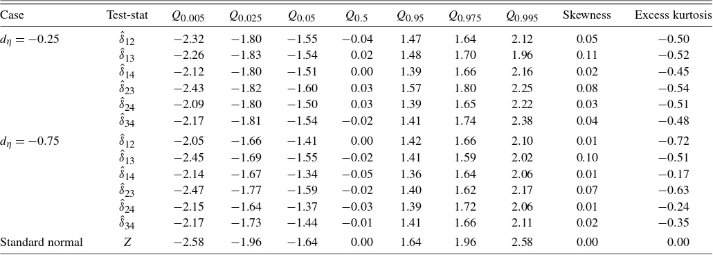
null hypothesis of normality is rejected at a nominal size of 1% based on the Kolmogorov–Smirnov goodness-of-fit test.
11. DATA ANALYSIS
In this section we focus on analyzing the buy prices,{P1,t},
and sell prices, {P2,t}, of a single stock, Tiffany Company
Table 2. Summary statistics of the simulation-based empirical distributions
Case Test-stat Q0.005 Q0.025 Q0.05 Q0.5 Q0.95 Q0.975 Q0.995 Skewness Excess kurtosis
dη= −0.25 δˆ12 −2.32 −1.80 −1.55 −0.04 1.47 1.64 2.12 0.05 −0.50
ˆ
δ13 −2.26 −1.83 −1.54 0.02 1.48 1.70 1.96 0.11 −0.52
ˆ
δ14 −2.12 −1.80 −1.51 0.00 1.39 1.66 2.16 0.02 −0.45
ˆ
δ23 −2.43 −1.82 −1.60 0.03 1.57 1.80 2.25 0.08 −0.54
ˆ
δ24 −2.09 −1.80 −1.50 0.03 1.39 1.65 2.22 0.03 −0.51
ˆ
δ34 −2.17 −1.81 −1.54 −0.02 1.41 1.74 2.38 0.04 −0.48
dη= −0.75 δˆ12 −2.05 −1.66 −1.41 0.00 1.42 1.66 2.10 0.01 −0.72
ˆ
δ13 −2.45 −1.69 −1.55 −0.02 1.41 1.59 2.02 0.10 −0.51
ˆ
δ14 −2.14 −1.67 −1.34 −0.05 1.36 1.64 2.06 0.01 −0.17
ˆ
δ23 −2.47 −1.77 −1.59 −0.02 1.40 1.62 2.17 0.07 −0.63
ˆ
δ24 −2.15 −1.64 −1.37 −0.03 1.39 1.72 2.06 0.01 −0.24
ˆ
δ34 −2.17 −1.73 −1.44 −0.01 1.41 1.66 2.11 0.02 −0.35
Standard normal Z −2.58 −1.96 −1.64 0.00 1.64 1.96 2.58 0.00 0.00