Full Terms & Conditions of access and use can be found at
http://www.tandfonline.com/action/journalInformation?journalCode=ubes20
Download by: [Universitas Maritim Raja Ali Haji] Date: 12 January 2016, At: 17:57
Journal of Business & Economic Statistics
ISSN: 0735-0015 (Print) 1537-2707 (Online) Journal homepage: http://www.tandfonline.com/loi/ubes20
Count Models Based on Weibull Interarrival Times
Blake McShane, Moshe Adrian, Eric T Bradlow & Peter S Fader
To cite this article: Blake McShane, Moshe Adrian, Eric T Bradlow & Peter S Fader (2008) Count
Models Based on Weibull Interarrival Times, Journal of Business & Economic Statistics, 26:3, 369-378, DOI: 10.1198/073500107000000278
To link to this article: http://dx.doi.org/10.1198/073500107000000278
Published online: 01 Jan 2012.
Submit your article to this journal
Article views: 106
View related articles
Count Models Based on Weibull
Interarrival Times
Blake M
CS
HANEDepartment of Statistics, Wharton School, University of Pennsylvania, Philadelphia, PA 19104
Moshe A
DRIANDepartment of Mathematics, University of Maryland, College Park, MD 20742
Eric T. B
RADLOWand Peter S. F
ADERDepartment of Marketing, Wharton School, University of Pennsylvania, Philadelphia, PA 19104 (ebradlow@wharton.upenn.edu)
The widespread popularity and use of both the Poisson and the negative binomial models for count data arise, in part, from their derivation as the number of arrivals in a given time period assuming exponentially distributed interarrival times (without and with heterogeneity in the underlying base rates, respectively). However, with that clean theory come some limitations including limited flexibility in the assumed un-derlying arrival rate distribution and the inability to model underdispersed counts (variance less than the mean). Although extant research has addressed some of these issues, there still remain numerous valuable extensions. In this research, we present a model that, due to computational tractability, was previously thought to be infeasible. In particular, we introduce here a generalized model for count data based upon an assumed Weibull interarrival process that nests the Poisson and negative binomial models as special cases. The computational intractability is overcome by deriving the Weibull count model using a polyno-mial expansion which then allows for closed-form inference (integration term-by-term) when incorporat-ing heterogeneity due to the conjugacy of the expansion and a commonly employed gamma distribution. In addition, we demonstrate that this new Weibull count model can (1) model both over- and underdis-persed count data, (2) allow covariates to be introduced in a straightforward manner through the hazard function, and (3) be computed in standard software.
KEY WORDS: Closed-form inferences; Hazard models; Polynomial expansions.
1. INTRODUCTION
The widespread popularity of the Poisson model for count data arises, in part, from its derivation as the number of arrivals in a given time period assuming exponentially distributed inter-arrival times. But of the thousands of other count models that have been developed over the years (see Wimmer and Altmann 1999 for an excellent synthesis), very few share this straightfor-ward connection between a count model and its timing model equivalent. The connection between a count model and a tim-ing process is more than just a theoretical nicety: in many dif-ferent contexts, it is useful—if not essential—for a researcher to be able to estimate a model using one form (timing or count-ing) but apply it using the other. As but one example, marketing managers frequently collect interarrival time data (often in the form of a recency question) but want to make predictions of the number of arrivals (purchases) that a particular customer is likely to make over the next year.
Furthermore, the Poisson count model is truly valid only in the case where the data of interest support the restrictive as-sumption ofequidispersion, that is, where the variance of the data equals the mean. Statisticians have recognized this limi-tation for many years, and now routinely use models that al-low foroverdispersion(i.e., datasets marked by a fatter, longer right tail than the Poisson can accommodate). A heterogeneous gamma-Poisson model (i.e., the negative binomial or NBD) is generally the first count model invoked for this common sit-uation. But what about datasets with the opposite problem, namely,underdispersion? Statisticians have acknowledged and addressed this issue in different ways (King 1989; Cameron and
Johansson 1997; Cameron and Trivedi 1998), but with the pos-sible exception of a count model featuring gamma-distributed interarrival times proposed by Winkelmann (1995), none of these underdispersed count models (to the best of our knowl-edge) offers the conceptual elegance and usefulness of the Poisson-exponential connection.
Winkelmann (1995) readily admitted the limitations of his gamma-based model. Among other reasons, he commented on the inability to obtain a closed-form hazard function for the gamma, which makes the incorporation of explanatory vari-ables an ad hoc process when compared to the standard Poisson or NBD “regression” models. He pointed out that “the Weibull distribution is preferred in duration analysis for its closed-form hazard function. . . ” but did not pursue such a model. The devel-opment and exploration of such a model is the main objective of the present article.
Before we develop our Weibull count model, we first set the stage by laying out the main properties that the Weibull count model developed here embodies.
(1) The model generalizes (nests) the most commonly used extant models such as the Poisson and the NBD as spe-cial cases; thus, when a simple structure is sufficient, the researcher will see it through the estimated model pa-rameters. Furthermore, standard inferential procedures
© 2008 American Statistical Association Journal of Business & Economic Statistics July 2008, Vol. 26, No. 3 DOI 10.1198/073500107000000278
369
(e.g., the likelihood ratio test) can be used to compare different specifications.
(2) The model handles both overdispersed and underdis-persed data, both of which are likely to be seen in prac-tice.
(3) Researchers who believe that the interarrival times of their dataset are Weibull distributed now have a corre-sponding counting model to use.
(4) The model is computationally feasible to work with: it is estimable without requiring a formal programming lan-guage or time-consuming simulation-based methods. (5) The model allows for the incorporation of person-level
heterogeneity reflecting the fact that individuals’ interar-rival rates may vary quite substantially across the popu-lation.
(6) The mechanism required to incorporate covariate effects is clear and simple. This process is consistent with stan-dard “proportional-hazards” methods, which represent the dominant paradigm for ordinary single-event timing models.
In this article we derive a new model for count data that sat-isfies these six criteria in the following ways. First, our count model is based upon an assumed Weibull interarrival process, which nests the exponential as a well-known special case. Sec-ond, we demonstrate that the Weibull count model, via the shape parameter being less than, equal to, or greater than 1, can capture overdispersed, equidispersed, and underdispersed data, respectively. Third, the Weibull interarrival time story is richer than the exponential story, because it allows for nonconstant hazard rates (duration dependence). Fourth, we implement the model entirely in standard software. This is accomplished by deriving our model using a polynomial expansion (which can be expressed in closed form). See Bradlow, Hardie, and Fader (2000), Everson and Bradlow (2002), and Miller, Bradlow, and Dayaratna (2006) for similar polynomial expansion solutions for the negative binomial, beta-binomial, and binary logit mod-els, respectively. Fifth, and related to the previous point, once the model is expressed as a closed-form sum of polynomial terms, we can easily introduce a conjugate mixing distribu-tion (the gamma distribudistribu-tion) to capture the underlying disper-sion in incidence rates across individuals. This ensures that our model nests the NBD in addition to the Poisson. Finally, we will demonstrate that we can use the proportional-hazards approach to introduce covariates in a very natural manner.
The remainder of this article is laid out as follows. In the next section, we provide a more detailed description of the ma-jor ways in which other researchers have extended basic count models (but rarely with an eye toward maintaining a known in-terarrival timing process). Section 3 contains the derivation of our Weibull count model, focusing on the polynomial expan-sion that leads to the closed-form benefits. In Section 4 we re-analyze the same data used by Winkelmann (1995) and provide a set of results comparing a sequence of nested models, the most complicated of which has an underlying Weibull arrival process, heterogeneous baseline rates, and covariates. Through the sequence of models that we fit, we are able to ascertain which aspects of the model are most critical. Finally, we pro-vide some concluding remarks and areas for future research in Section 5.
2. PRIOR RELATED RESEARCH
The primary way in which this research contributes to the literature on count data is by generalizing the underlying in-terarrival timing model to allow for greater flexibility in its hazard function, which is how flexible forms of dispersion are accounted for (as described later). For example, Winkelmann (1995) offered a careful analysis of a counting model based on gamma-distributed interarrival times and discussed the relation-ship between the nature (i.e., slope) of the timing model hazard function and the type of dispersion seen in the equivalent count data. In particular, if we denote the mean of the interarrival dis-tribution byμ, the variance byσ2, and the hazard function by
h(t)= f(t)
1−F(t),
wheref(t)andF(t)are the density and cumulative probability functions, respectively, we say that the distribution has negative duration dependence ifdh(t)/dt<0 and positive duration de-pendence ifdh(t)/dt>0. If the hazard function is monotonic, then
(see Barlow and Proschan 1965, p. 33). These three cases corre-spond to count data characterized by underdispersion, equidis-persion, and overdisequidis-persion, respectively.
Focusing on nonconstant hazard rates (as above) is but one way in which researchers have extended count models; we dis-cuss some other methods briefly. Another way to capture the same kinds of patterns seen in duration-dependent models is to assume that the probability of an event occurring depends on the number of eventsthat have occurred previously, as opposed to thearrival timeof the most recent event (duration dependence). These models are said to display contagion. For instance, they have been studied in the literature on accident proneness (Ar-bous and Kerrich 1951; Feller 1943). For more information, one can reference Gurland and Sethuraman (1995) for a con-tagious discrete- time model that leads to the negative binomial in which an occurrence increases and a nonoccurence decreases the probability of a future occurrence. Other models for oc-currence dependence have been developed by Mullahy (1986) and Gourieroux and Visser (1997). One can also make the as-sumption that successive events are independent but the process intensity varies as a function of time. This class of models is known as nonhomogeneous Poisson processes and is described in Lawless (1987). We believe that a promising area for future research would be a comparison of both forms of dependence (duration and occurrence), although here we focus only on the former.
Beyond an explicit focus on any kind of time dependence, there are many other distributions that have been formulated to be able to accommodate underdispersed as well as overdis-persed data. Researchers such as Bening and Korolev (2002), Cameron and Trivedi (1998), King (1989), and Shmueli,
McShane et al.: Count Models 371
Minka, Kadane, Borle, and Boatwright (2005) have proposed and discussed a wide variety of generalized count models that can handle overdispersion and underdispersion. But few (if any) offer the benefits or elegance of something like the Poisson-exponential connection. In the next section we lay out our model that fully respects this connection and also offers a great deal of flexibility in being able to capture a range of count data dispersion patterns.
2.1 A Modeling Framework
Much extant research on count data has been focused on ex-tending the basic Poisson model (denoted here as model [0]) to allow for hyperdispersion via a nonconstant hazard rate. The basic ways in which hyperdispersion has been accounted for in-clude (model [1]) adding covariates to the model, (model [2]) incorporating individual-level heterogeneity for the baseline rates, and (model [3]) both [1] and [2]. In particular, if we let
[Xit|λi] ∼Poisson(λiexp(Zit′β)), (1)
a proportional-hazards framework (Cox 1972), where Xit is
a nonnegative integer (count) for unit i=1, . . . ,I on its t=
1, . . . ,Tith observation, λi is the baseline rate for uniti,Zit= (Zit1, . . . ,ZitP)is a vector of covariates that describe each
in-dividual, andβ′=(β
1, . . . , βP)is a vector of covariate slopes:
model [0] is obtained by settingλi=λfor alliandZit′β=0 (an
intercept only); model [1] is obtained by settingλi=λfor alli
(the Poisson regression model); model [2] is obtained by setting P=1,Zitβ=0 and lettingλi∼g(λi|θ )(whengis the gamma
distribution, then model [2] integrated over the distribution of
λi is the negative binomial distribution); and model [3] is as
given in (1) where againλi∼g(λi|θ ). Model [3] is also
some-times referred to as the NegBin II model or a random-intercepts Poisson regression model. Later in Section 4, we compare the results of models [0]–[3] to those derived in this research.
What is of interest to note is that all of these extensions use the Poisson model (with associated exponential interarrival times) as their kernel. That is, these extensions to the model have not been done at the core unit of analysis, that is, the un-derlying arrival time distribution, but instead work strictly with the count model. What we do in this research is to enhance the flexibility of the arrival time model to account for richer pat-terns. In particular, instead, we assume that the underlying ar-rival time distribution forYik, thekth arrival for uniti, follows
a Weibull distribution with density given by
f(Yik=y|λi, β,c)=λicyc−1exp(−λiyc). (2)
Later, when we introduce covariates into the model, we do it through the hazard function:
h(t)=λctc−1, (3)
which is monotonically increasing forc>1, monotonically de-creasing forc<1, and constant (and equal toλ) whenc=1.
Using the standard proportional-hazards framework, we then boost this “baseline” hazard [given in (3)] by a weighted vec-tor of the covariatesh(t)=h0(t)exp(β′Z), and then rely on the well-known relationship between the hazard function and the cdf:
F(t)=1−exp
−
(h(u)du)
to arrive at the Weibull regression model
f(Yik=y|λi, β,c)=λiexp(Zit′β)cyc−1exp
−λiexp(Zit′β)yc
.
(4)
We note that whenc=1, (4) simplifies to a heterogeneous exponential arrival time model with covariates that leads to count models [0]–[3] above.
Thus, directly analogous to models [0]–[3] which are based on an exponential interarrival time, our interest lies in looking at various reduced-form specifications of the model given in (4). Specifically, we denote as model [4] the Weibull model without heterogeneity and without covariates (model [0] analog) such thatλi=λandZit′β=0. We label model [5] as the Weibull
re-gression model (without heterogeneity) such thatλi=λ. Model
[6] is the model (to be discussed in Sec. 3.2) in which we allow for heterogeneity in baseline ratesλibut do not include
covari-ates (Z′itβ =0). Finally, model [7] is the fully parameterized model that includes heterogeneity and covariates. All eight of these models will be fit and results compared in Section 4.
It is important to note that whereas the baseline Weibull model proposed here in (3) allows for increasing, constant, or decreasing hazard, the individulevel hazard function is al-ways monotonic. The way in which this restriction is addressed here is via the inclusion of time-varying covariates,Zit, as in (4),
and with the gamma mixing distribution. These additions pro-vide a great deal of flexibility to accommodate virtually any kind of observable (i.e., aggregate) hazard function. Alterna-tively, one can start with a nonmonotonic hazard function at the individual level, for example, using a generalized Weibull model (Mudholkar, Srivastava, and Kollia 1996). Whereas such a distribution would provide even greater flexibility, we are cau-tious about taking this step. When heterogeneity and/or covari-ates are also included in the model, it becomes difficult to sort out the various effects, and computational concerns arise as well. Our experience suggests that there is already enough flex-ibility with the proposed model, and further generalizations— involving difficult trade-offs between modeling flexibility, pa-rameter identification, and data requirements—should be ap-proached with great care.
3. BASIC THEORY AND DEFINITIONS
Before discussing the Weibull count model itself, we de-scribe the general framework utilized to derive the model that is based upon the relationship between interarrival times and their count model equivalent. LetYnbe the time from the
mea-surement origin at which thenth event occurs. LetX(t)denote the number of events that have occurred up until timet. The re-lationship between interarrival times and the number of events is
Yn≤t ⇔ X(t)≥n.
We can restate this relationship by saying that the amount of time at which the nth event occurred from the time origin is less than or equal totif and only if the number of events that have occurred by timetis greater than or equal ton.
We therefore have the following relationships that allow us the measurement time origin (and thus the counting process) coincides with the occurrence of an event, thenFn(t)is simply
then-fold convolution of the common interarrival time distribu-tion which may or may not have a closed-form soludistribu-tion. Based upon (5), we derive our Weibull count model next based upon a polynomial expansion ofF(t).
3.1 Weibull Count Model
We derive the basic Weibull count model, model [4] from ear-lier, by assuming that the interarrival times are independent and identically distributed Weibull with probability density func-tion (pdf) f(t)=λctc−1e−λtc (c, λ∈R+), and corresponding cdfF(t)=1−e−λtc, which simplifies to the exponential model whenc=1.
The challenge in deriving the Weibull count model arises in the need to be able to evaluate convolutions of the form
t
0F(t−s)f(s)ds. Whereas this integral is easily solved for the exponential density as well as the gamma with an integer-value shape parameter (a.k.a. the Erlang distribution), it does not have a proper solution for the Weibull. Thus, our approach is to han-dle this integral (and derive the Weibull count model as a whole) using a Taylor series expansion of the Weibull density.
In particular, the Taylor series approximations obtained by expanding the exponential pieces (eλtc), respectively, for both the cdf and pdf of the Weibull are
F(t)= the following recursive relationship that we utilize in deriving the Weibull count model:
Before proceeding to develop the general solution to the problem, we note that F0(t) is 1 for all t and F1(t)=F(t).
McShane et al.: Count Models 373 Therefore, we have the main result of this article, the Weibull count model:
We note in addition that the expectation of this count model is
In fact, the moment generating function (MGF) is also read-ily obtained. In particular, letMI(u)denote the MGF whereIis
the Weibull counting random variable in the pdf. Then,
MI(u)=E(eiu)
and correspondingly, to obtain the moments we note that
dn
Hence, based on our polynomial expansion, we obtain closed-form expressions for the density as well as its moments.
3.2 The Benefits of the Weibull Count Model
We now revisit the properties listed in Section 1, point by point (and provided in italics below), to describe both those as-pects that the basic Weibull count model (without covariates and without heterogeneity) given in (11) provides, and those that require extensions.
(1) The model generalizes (nests) the most commonly used extant models such as the Poisson and the NBD as special cases; thus, when a simple structure is suffi-cient, the researcher will clearly see it through the es-timated model parameters. Furthermore, standard infer-ential procedures (e.g., the likelihood ratio test) can be used to compare different specifications.
We note that when we set c=1 and t =1 in (11), we do in fact get the Poisson count model as P(N(t)=n)=
∞
j=n(−1)j+n(λ)jαnj/Ŵ(j+1), a standard result. With regard
to the negative binomial model, we discuss this with respect to item 5 below, whenλis allowed to vary across the population.
(2) The model handles both overdispersed and
underdis-persed data, both of which are likely to be seen in prac-tice.
Through extensive simulations (because the result is unavail-able in closed form), we have verified that for 0<c<1, the probability mass function associated with the Weibull count model displays overdispersion, whereas forc>1, underdisper-sion is displayed. That is, the underlying interarrival times have a decreasing (increasing) hazard for 0<c<1 (c>1). Thus, negative duration dependence is associated with overdispersion, positive duration dependence with underdispersion (Winkel-mann 1995). A lack of duration dependence leads to the Poisson distribution with equal mean and variance.
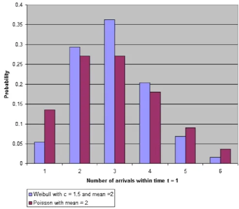
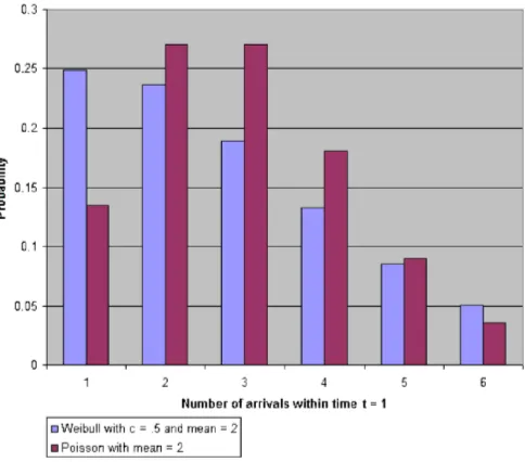
As one demonstration of these findings, Figures 1 and 2 dis-play probability histograms for the Weibull and Poisson count models with different parameter values. Both the Weibull and the Poisson were intentionally chosen to have identical means
Figure 1. Poisson and Weibull models displaying underdispersion.
Figure 2. Poisson and Weibull models displaying overdispersion.
(set to 2); yet their dispersion is quite different. In Figure 1, we have the probability histograms for an underdispersed Weibull with parameters c=1.5 and λ=2.93, and a Poisson with
λ=2. The variance of the Weibull count model in this case is .880. In Figure 2, we have the probability histograms for an overdispersed Weibull with parameters c=.5 and λ=1.39, and again the Poisson withλ=2. The variance of the Weibull count model in this case is 3.40, which is greater than the mean, as expected.
(3) Researchers who believe that the interarrival times of their dataset are Weibull distributed now have a corre-sponding counting model to use.
As (11) is derived from the Weibull timing model, the link between the timing model and its counting model equivalent is maintained. Hence, in those cases where an analysis of the interarrival times (if the data are available) suggests that a more flexible timing model is needed, it can now be incorporated via its count model equivalent. Furthermore, in those cases where one only has count data, but would like to make forecasts of the next arrival time, this can now be done given the timing and count model link that is now achieved.
(4) The model is computationally feasible to work with: it is estimable without requiring a formal programming lan-guage or time-consuming simulation-based methods.
Although the summations shown in the expressions above may seem a bit daunting at first, they are easy to manage from an operational standpoint. We will demonstrate in Section 4 that the model is tractable enough that we perform parameter esti-mation in standard software, and in addition that the results are not particularly sensitive to the number of terms that are used in the summation, beyond a certain point, which can be identified through empirical testing.
(5) The model allows for the incorporation of person-level heterogeneity reflecting the fact that individuals’ interar-rival rates may vary quite substantially across the popu-lation.
One nice feature of the model presented in (11) is that in-troducing heterogeneity across units in their rate parameters,
λi, is straightforward. If, as is standard in many timing models,
we assume that the underlying rates are drawn from a gamma distributionλi∼gamma(r, α), we can increase the model
flex-ibility at the expense of only one additional model parameter and also, as per item 1, when c=1 nest the negative bino-mial model. Thus, when we combine our polynobino-mial expansion Weibull count model in (11) with a gamma mixing distribution, we get a count model that nests the Poisson and negative bino-mial.
In particular, the derivation of the heterogeneous Weibull count model, model [6] from Section 2.1, is given as follows:
P(N(t)=n)=
This expression is simply a weighted sum of thejth moments of the gamma distribution around zero,Ŵ(r+j)/Ŵ(r)αj, asλji
enters the polynomial approximated likelihood in a linear way. Hence, the conjugacy of the gamma mixing distribution and the polynomial approximated likelihood is directly obtained.
(6) The mechanism required to incorporate covariate effects is clear and simple. This process is consistent with stan-dard “proportional-hazards” methods, which represent the dominant paradigm for ordinary single-event timing models.
Now that we have the closed-form solution for the hetero-geneous count model with an underlying Weibull interarrival process, we extend it to allow for the inclusion of covariates, that is, models [5] and [7] from Section 2.1. We define the Weibull regression model, without heterogeneity, as
P(N(t)=n)=
wherex′i denotes the covariate vector for unitiandβ a set of covariate slopes. In an analogous manner, we derive model [7], our most complex model which allows for Weibull interarrival times, covariate heterogeneity, and parameter heterogeneity and is given by
McShane et al.: Count Models 375
after integrating overλi∼gamma(r, α).
We next describe an application of these models using a dataset initially described and analyzed by Winkelmann (1995) that is an underdispersed count dataset with covariates.
4. TESTING AND RESULTS
Besides the derivation of the Weibull count model, and the extensions to include covariates and heterogeneity, an addi-tional goal of this research was to provide an empirical demon-stration of our model. Is the polynomial expansion derived here empirically tractable, and will it provide improved results com-pared to existing methods? Remarkably enough, the tional approach for our class of models, including the computa-tion of bootstrap standard errors (Efron 1982), was conducted entirely in Microsoft Excel, an aspect we believe makes our ap-proach widely accessible. The spreadsheet calculates the first hundredαcoefficients, and then uses Solver to maximize the likelihood with respect to the data; it is available upon request. Specifically, to compute the standard errors of coefficients under the series of models, we utilized a bootstrap procedure in which 100 replicate datasets of identical size to the origi-nal data for each model were generated by sampling individ-ual respondent covariate-count outcome pairs, (Zi,Ni), with
re-placement. The results reported for the standard errors are the standard deviation of the coefficients across those samples. We note that the bootstrapping procedure can be implemented using a weighted likelihood approach where each observation pair’s weight in the likelihood is the number of times that it appears in the replicate sample. This equivalence of using a weighted likelihood approach to compute bootstrap standard errors is not specific to this model, so it can be utilized in a large number of research domains, and can be applied in software packages (e.g., a spreadsheet) that contain little more than random num-ber generation and function maximizing capabilities. In addi-tion, bootstrap standard errors were compared to standard er-rors computed using numerical estimates of the gradient and Hessian. The standard errors were of comparable magnitude in all cases, contained no general pattern, and were roughly 20– 30% bigger on average using the bootstrap, reflecting the po-tential asymmetric and heavier tailed models utilized here.
We apply our series of models to a dataset initially (and more fully) described by Winkelmann (1995) which contains as a dependent variable the number of children born to a random sample of females. A number of explanatory variables,Zi, are
available including the female’s general education (measured
as the number of years of school), a series of dummy variables for post-secondary education (either vocational training or uni-versity), nationality (German or not), rural or urban dwelling, religious denomination (Catholic, Protestant, and Muslim, with other or none as reference group), and continuous variables for year of birth and age at marriage.
This dataset was chosen for a number of reasons. First, the article by Winkelmann (1995) acted as a motivation for this re-search; hence utilizing the identical dataset made sense. Sec-ond, for this dataset, the variance of the number of births is less than the mean (2.3 versus 2.4); thus we have an opportunity to demonstrate the ability of the Weibull family of count models to handle underdispersion. Finally, as Winkelmann (1995) already contained the results for the Poisson regression model (model [1] here) and the gamma-based count model that he derived in that article, we already had results that would both let us con-firm the accuracy of our computational approach and provide a strong benchmark (the gamma-based model) to which we can compare the Weibull.
Before presenting the results, we note (as is standard in ex-tant Weibull timing model research) that we reparameterized our Weibull count model from its regular form(r, α,c)to a pa-rameterization given by(1/r,r/α,c). This has been shown to have (and we confirm here that there are) multiple benefits in model implementation, including (1) greater stability in the pa-rameter estimation process, (2) papa-rameter estimates that are not at the boundary of the parameter space (thus enabling likeli-hood ratio tests for model comparison), and (3) standard errors of coefficients that are more stable and meaningful than those associated with the direct estimation ofr, α, andc.
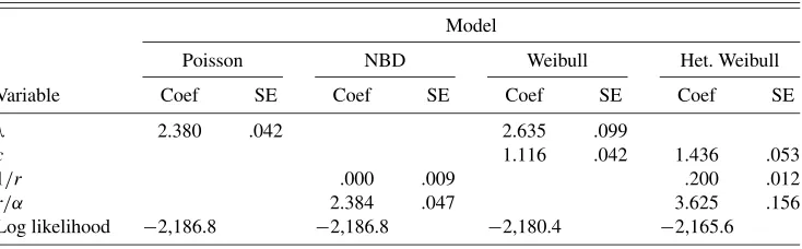
Tables 1 and 2 list the results of the basic models (without covariates) and the regression models, respectively. We note that the log-likelihood values computed using our count model approach, for both the regular Poisson (LL= −2186.8) and Poisson regression (LL= −2101.8), are identical to those in table 1 of Winkelmann (1995, p. 471), thus verifying the ac-curacy of our polynomial expansion approach. In addition, the last column in Table 2, the results of the gamma count regres-sion model, is taken directly from table 1 of Winkelmann (1995, p. 471). We describe our findings with respect to the models first without and then with covariates.
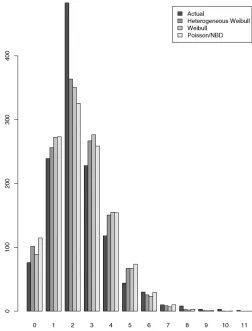
In Figure 3 we plot the actual and fitted values for the Pois-son, the NBD, the Weibull, and the heterogeneous Weibull, not-ing that, for this dataset, the Poisson and the NBD are indistin-guishable. Whereas all of the models tend to underfit at two children and overfit for values near two, a result also seen in
Table 1. Basic model results for total marital fertility
Model
Poisson NBD Weibull Het. Weibull
Variable Coef SE Coef SE Coef SE Coef SE
λ 2.380 .042 2.635 .099
c 1.116 .042 1.436 .053
1/r .000 .009 .200 .012
r/α 2.384 .047 3.625 .156
Log likelihood −2,186.8 −2,186.8 −2,180.4 −2,165.6
Table 2. Regression model results for total marital fertility
Model
Poisson NBD Weibull Het. Weibull Gamma
Variable Coef SE Coef SE Coef SE Coef SE Coef SE
German −.200 .050 −.198 .040 −.229 .062 −.268 .054 −.190 .060
Years of schooling .033 .004 .034 .002 .038 .010 .062 .015 .032 .027
Vocational training −.153 .038 −.152 .033 −.173 .047 −.181 .040 −.144 .037
University −.155 .098 −.155 .087 −.179 .125 −.264 .076 −.146 .130
Catholic .218 .046 .218 .042 .244 .066 .242 .038 .206 .059
Protestant .113 .057 .113 .043 .125 .069 .118 .046 .107 .063
Muslim .548 .064 .551 .052 .640 .089 .673 .037 .523 .070
Rural .059 .031 .062 .027 .068 .038 .071 .042 .055 .032
Year of birth .002 .001 .003 .000 .002 .001 .003 .003 −.002 .002
Age at marriage −.030 .003 −.030 .000 −.030 .003 −.034 .006 −.290 .006
λ 3.150 .264 4.050 .331
c 1.236 .045 1.362 .061
1/r .000 .000 .061 .008
r/α 3.130 .131 3.604 .093 1.439 .233
Log likelihood −2,101.8 −2,101.8 −2,077.0 −2,067.5 −2,078.2
Winkelmann (1995) even when covariates were included, the heterogeneous Weibull minimizes error and maximizes likeli-hood. Given that the location of the error falls at the value of two children, a number of children seen as ideal by many, and this error seems consistent across models, we might con-clude that contraceptive practices or cultural norms have
“in-Figure 3. Fertility data compared to fitted values.
terfered” with the underlying independence and identically dis-tributed assumption. Moreover, we would expect the Weibull models to perform best relative to the Poisson and the NBD on datasets that are underdispersed, which it does. However, for this dataset, the mean is 2.4 and the variance is 2.3, so the data are only very slightly underdispersed, thus explaining the simi-larity of the fitted values.
The basic models show that both Weibull count models have significantly better log-likelihoods than the Poisson and the NBD. The latter two models are identical for this dataset, be-cause the observed underdispersion will drive the NBD hetero-geneity to zero (the corresponding values ofrandαobtained from 1/randr/αare extremely large). The presence of gamma heterogeneity around the Poisson process would overdisperse, not underdisperse, the fertility counts, so it would not help in this case. Interestingly, once one utilizes the Weibull timing model instead of the exponential, the need for heterogeneity now arises (LL= −2165.5 for the heterogeneous Weibull as compared to−2180.4 for the nonheterogeneous). In fact, we hypothesize that because the Weibull model indicates duration dependence (csignificantly greater than 1), this needs to be counterbalanced by heterogeneity to provide an adequate fit. It is somewhat unusual to encounter a situation in which the move to a more flexible individual-level model leads to a greater de-gree of heterogeneity than a more restricted specification. Al-though we observe this pattern for our data, we do not know if it holds in general; it is an interesting area for future research.
The results in Table 1 provide initial evidence that duration dependence plays a distinctly different role when compared to heterogeneity. It is valuable to have a model that can distinguish between these two factors. If the underlying dataset were in-stead overdispersed, one could use the heterogeneous Weibull count model to determine whether the “non-Poisson” disper-sion effects were coming from the underlying timing process or from cross-sectional differences. This can be a valuable contri-bution of our model.
Notice finally that the value ofc in the nonheterogeneous Weibull model is 1.116, slightly more than two standard errors
McShane et al.: Count Models 377
above 1.0, and for the heterogeneous model it is 1.436—almost eight standard errors above 1.0. This is consistent with our ear-lier discussion result that whencis greater than 1, the Weibull count model’s variance is less than the mean—underdispersion. It also indicates that the “arrival process” for babies is not com-pletely random. A mother is unlikely to have a baby immedi-ately after the birth of a previous child (which fits the laws of nature quite well), but the odds (or hazard) of delivering another child steadily increase thereafter. An anonymous reviewer sug-gested that a Weibull model with a “blocked” period reflecting that women cannot have children within a certain time frame after birth would be a more realistic empirical model, and we agree that this is an interesting area for future research.
Turning our attention to the models with covariates, we first note that the two Weibull regression models provide the best fits, that is, a slight improvement in log-likelihood for the Weibull model without heterogeneity and a significant improve-ment for the heterogeneous Weibull model, compared to the Poisson and Winkelmann’s gamma count model. The values ofcfor the Weibull regression and heterogeneous Weibull re-gression models are comparable to the models with no covari-ates, and still significantly greater than 1.0. The coefficients for the covariates show very small differences across the models. The coefficients of all variables are identical in sign to those in Winkelmann (1995), are extremely stable across the class of models, and have comparable standard errors such that the variables that are significant coincide in both sets of models (the only difference of note is that the year-of-birth and age-of-marriage variables were centered in Winkelmann, and not here, hence the difference in size of the coefficients; the Pois-son regression models as indicated by the log-likelihoods are the same).
5. CONCLUSIONS
In this research, we have derived and provided an empirical demonstration for an entirely new class of count models de-rived from a Weibull interarrival time process. The new model has many nice features such as its closed-form nature, compu-tational simplicity, the ability to nest both the Poisson and NBD models, and the ability to bring in both heterogeneity and co-variates in a natural way. The key to the derivation is the use of a Taylor series expansion to get around the fact that, unlike the exponential or gamma distributions, there is no simple way to obtain a convolution of two (or more) Weibulls.
From an empirical standpoint, we showed that the Weibull count model without heterogeneity offers a slight improvement in log-likelihood when compared to the gamma count model of Winkelmann (1995) and a dramatic improvement over ex-tant models commonly used. When including heterogeneity in the Weibull model (both with and without covariates), the im-provement is even greater, suggesting that the improved ef-fects of adding a flexible timing model and heterogeneity may be complementary. Admittedly it is impossible to generalize from one dataset, but these results provide encouraging signs about the model’s validity and usefulness. More importantly, the model provides a sizeable improvement over the more tradi-tional Poisson/NBD model (with and without covariates). This may have important implications in many cases, because most
researchers have always turned to heterogeneity as the first ex-planation/correction for datasets that do not conform well to the simple assumption of Poisson counts (and, implicitly, exponen-tial interarrival times). Now researchers have a very plausible second explanation available (i.e., Weibull interarrival times) and they can further explore it using conventional techniques such as proportional hazards for covariates and a parametric mixing distribution for heterogeneity. This is a powerful com-bination of old and new methods that has substantial promise for a wide variety of application areas.
ACKNOWLEDGMENT
The authors thank Rainer Winkelmann for useful suggestions and comments and for generously providing us the data used in this study.
[Received January 2006. Revised February 2007.]
REFERENCES
Arbous, A. G., and Kerrich, J. E. (1951), “Accident Statistics and the Concept of Accident-Proneness,”Biometrics, 7, 341–433.
Barlow, R. E., and Proschan, F. (1965),Mathematical Theory of Reliability, New York: Wiley.
Bening, V. E., and Korolev, V. Y. (2002),Generalized Poisson Models and Their Applications in Insurance and Finance, Leiden, Netherlands: Brill Academic Publishers.
Bradlow, E. T., Hardie, B. G. S., and Fader, P. S. (2002), “Bayesian Inference for the Negative Binomial Distribution via Polynomial Expansions,”Journal of Computational and Graphical Statistics, 11, 189–201.
Cameron, A. C., and Johansson, P. (1997), “Count Data Regression Using Se-ries Expansion: With Applications,”Journal of Applied Econometrics, 12, 203–223.
Cameron, A. C., and Trivedi, P. K. (1998),Regression Analysis of Count Data, Cambridge, U.K.: Cambridge University Press, pp. 59–188.
Cox, D. R. (1972), “Regression Models and Life-Tables,”Journal of the Royal Statistical Society, Ser. B, 34, 187–220.
Efron, B. (1982), “Bootstrap Methods: Another Look at the Jackknife,”The An-nals of Statistics, 7, 1–26.
Everson, P. J., and Bradlow, E. T. (2002), “Bayesian Inference for the Beta-Binomial Distribution via Polynomial Expansions,”Journal of Computa-tional and Graphical Statistics, 11, 202–207.
Feller, W. (1943), “On a General Class of ‘Contagious’ Distributions,”The An-nals of Mathematical Statistics, 14, 389–400.
Gourieroux, C., and Visser, M. (1997), “A Count Data Model With Unobserved Heterogeneity,”Journal of Econometrics, 79, 247–268.
Gurland, J., and Sethuraman, J. (1995), “How Pooling Failure Data May Re-verse Increasing Failure Rates,”Journal of the American Statistical Associa-tion, 90, 1416–1423.
King, G. (1989), “Variance Specification in Event Count Models: From Restric-tive Assumptions to a Generalized Estimator,”American Journal of Political Science, 33, 762–784.
Lawless, J. F. (1987), “Regression Methods for Poisson Process Data,”Journal of the American Statistical Association, 82, 808–815.
Miller, S. J., Bradlow, E. T., and Dayaratna, K. (2006), “Closed-Form Bayesian Inferences for the Logit Model via Polynomial Expansions,”Quantitative Marketing and Economics, 4, 173–206.
Mudholkar, G. S., Srivastava, D. K., and Kollia, G. D. (1996), “A Generaliza-tion of the Weibull DistribuGeneraliza-tion With ApplicaGeneraliza-tion to the Analysis of Survival Data,”Journal of the American Statistical Association, 91, 1575–1583. Mullahy, J. (1986), “Specification and Testing of Some Modified Count Data
Models,”Journal of Econometrics, 33, 341–351.
Shmueli, G., Minka, T. P., Kadane, J. B., Borle, S., and Boatwright, P. (2005), “A Useful Distribution for Fitting Discrete Data: Revival of the Conway– Maxwell–Poisson Distribution,” Journal of the Royal Statistical Society, Ser. C, 54, 127–142.
Trivedi, P. K., and Cameron, A. C. (1996), “Applications of Count Data Models to Financial Data,” inHandbook of Statistics, Vol. 14, Amsterdam: North-Holland, Chap. 12, pp. 363–391.
Trivedi, P. K., and Deb, P. (1997), “The Demand for Health Care by the Elderly: A Finite Mixture Approach,”Journal of Applied Econometrics, 12, 313–332. Wimmer, G., and Altmann, G. (1999),Thesaurus of Univariate Discrete
Prob-ability Distributions, Germany: Stamm Verlag.
Winkelmann, R. (1995), “Duration Dependence and Dispersion in Count-Data Models,”Journal of Business & Economic Statistics, 13, 467–474.
(2003),Econometric Analysis of Count Data(4th ed.), Heidelberg, NY: Springer.