The Influence of Decadal Kelvin Wave into 22oC Isotherm Depth along Western of Sumatra and Southern of Java by Using Wavelet Coherence
Hanah Khoirunnisa1, Nining Sari Ningsih2, Fadli Syamsudin3 1State Polytechnic of Batam, Batam, Indonesia
2Bandung Institute of Technology, Bandung, Indonesia
3Agency for the Assessment and Application of Technology (BPPT), Jakarta , Indonesia
1Email: [email protected]
Abstract
This study tried to observe the impact of the decadal Kelvin wave to the variation of thermocline depth along the western of Sumatra and southern of Java. The data would be used was the sea surface height anomaly (SSHA) data, sea temperature for 64 years (1950 – 2013), and Indian Ocean Dipole (IOD) index and Ocean Nino Index (ONI) for 54 years. They were the results of the 3D hydrodynamic models of HYbrid Coordinate Ocean Model (HyCOM). The used methods to analyze the effect of the decadal Kelvin wave to the thermocline depth variability were determination of the isotherm depth of T=22oC, S-transform to observe the energy spectrum and the period of isotherm depth of T=22oC change, and the last method was the wavelet coherency to prove the coherence between SSHA and the isotherm depth of T=22oC. The SSHA data and the isotherm depth of T=22oC has a correlation value of 0.7 with a 95% confidence level. It was reinforced by
the results of the wavelet coherence that showed a coherency between SSHA and isotherm depth of T=22oC with a period of 7.25 years (decadal) at any point that coincides with the occurrence of the decadal Kelvin wave along west of Sumatra and southern Java. The isotherm depth T=22oC has the variety of value at A to H point and its period were 8 to 11 years. In addition, when the decadal Kelvin wave propagated, the SSHA condition had been increasing while the isotherm depth of T=22oC had been decreasing.
Keywords: decadal varia bility, sea surface height anomaly, decadal Kelvin wave, Isotherm depth T= 22oC, wavelet coherence
Introduction
There were several variabilities of ocean-atmosphere interaction in Indian Ocean, they were: intra-seasonal, seasonal, inter-annual, decadal, and inter-decadal (Susanto et al, 2001; Syamsudin et al, 2004; Khoirunnisa et al, 2016). The one of the period of inter-annual changes in sea level that is affected by the climatic phenomenon in the Western Indian Ocean (Mahongo et al., 2014). Pacific Decadal Oscillation (PDO) has been observed in the Pacific Ocean and it has the two phases, such as the cold and warm phases (Mantua and Hare, 2002). The meteorology dominantly affects the decadal variability of the ocean-atmosphere interaction (Mahongo et al., 2014).
interactions in a large basin of the Indian Ocean that was derived from the monthly SST and surface wind data (Qian et al., 2001). The interannual variability of Indian Ocean dipole (IOD) has also the decadal modulation, moreover influenced the global cimate (Yuan et al., 2008). Additionally, the SSHA along the southern of Java has also the decadal (Khoirunnisa et al, 2015).
The Pacific and Indian Ocean have been influenced the Indonesian sea, the one of these was to deepening (shallowing) the thermocline depth (Wyrtki, 1961; Gordon, 1984; Gordon et al, 1994). Discovering the correlation between the variation of thermocline depth and IOD index has been proven (Ashok et al., 2004; Schott et al., 2009). The analysis has been done by Gordon et al. (1994) which showed that the water masses of Indian or the Pacific Ocean has influenced the thermocline in the Banda Sea. When the water mass of the Pacific Ocean was flowing to the Indian Ocean, the Banda seas thermocline has changed. The change of the thermocline depth variation in Indian Ocean has the seasonal variability. In addition, this correlated negatively to the sea level (Bray et al, 1996). The thermocline is the transition layer which connecting the warm masses water to the cool masses water (NOAA, 2017).
Similarity with the IOD index modulation, the decadal variability of the sea surface height (SSH) in the Indian ocean has also been observed in 1992 and 2001 as well as in the period 2001 to 2008 (Church et al., 2004; Han et al., 2008). In addition, the North Indian Ocean and the South Indian Ocean have been first observed decadal variability on the sea surface temperature anomaly (SSTA) during 1961 to 2000 (Han et al., 2008). The Tropical Indian Ocean region has also an important role on the climate. Based on the research by Han et al. (2008) stated that the thermocline depth and the heat content in the Indian Ocean tropical have the decadal variability in 1992 until 2008. Therefore, in the Indian Ocean has observed a link between atmospheric circulation and monsoon or the precipitation anomalies (Qian et al., 2001).
From the research that has been done by Khoirunnisa et al. (2016), there was a propagation of the decadal Kelvin wave as much as three times along the western of Sumatra and southern of Java during 1974 to 1976 and 1985 to 1985 and 1998 to 2001 with the period of 7.25 to 19.25 years. Based on the previous study, we would like to investigate the effect of a Kelvin wave to the thermocline depth variation along the western of Sumatra and Southern of Java. The used methods were the S-transform, wavelet coherence, and the determination of the isotherm depth T=22oC by using visual analysis diagram Hovmoller.
Data and Methods
and
http://www.cpc.ncep.noaa.gov/products/analysis_monitoring/ensostuff/ensoyears.shtml.
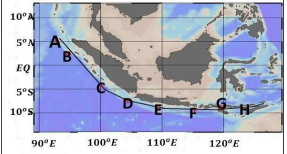
Figure 1 The study area to observe the influence of the decadal Kelvin wave into the variation of thermocline depth. The A – H point were the observation sample points.
The determination of the T=22oC isotherm depth has been done in along western of
Sumatra and southern of Java as a first step in this research. The thermocline depth was determined by the vertical distribution of the sea temperature. Susanto et al. (2001) determined the thermocline depth as well as at the T=22oC isotherm depth
(midthermocline). After that, S-transform was used to show the spectrum energy and the dominant period of the T=22oC isotherm depth variation. In order to determine the relationship between the decadal Kelvin wave and the thermocline depth variation, can be done by the correlation and coherence methods between them.
1. The Determination of T=22oC Isotherm Depth
The depth of the thermocline was determined from the vertical distribution of sea temperature data. Based on the research of Susanto et al. (2001), the thermocline depth was determined by the T=22oC isotherm depth, represented as the midthermocline.
The monthly averaged was applied to the T=22oC isotherm depth. Therefore, the seasonally variation could be observed. Figure 2 explains the illustration of the determination of the T=22oC isotherm depth which was considered as a midthermocline (Susanto et al., 2001).
2. S-transform
The second method was the s-transform to show the energy spectrum of the T=22oC
isotherm depth variation. S-transform was a window variable of Short Time Fourier Transform (STFT) or an extension of the Wavelet Transform (WT) (Wang, 2010). The Fourier transform only containing the information of the time-series spectrum components, however can not to detect the time distribution at the different frequencies. The wavelet transform either to extract information from the data with the time and frequency domains. However, the wavelet transform is sensitive to noise. Equation 1 shows the relationship of s-transform with STFT. Here is the STFT equation of the ℎ � signal:
� �, = ∫ ℎ �∞ � − � − � �
The S-transform can be determined by changed of � value into this followed Gaussian function in the Equation 1:
This method was applied to determine the T=22oC isotherm depth variation. Both of the raw data and the low-pass filter data by cut-off 3 years spectrum energies, these were observed by this method.
3. Wavelet Coherence
The wavelet coherence was used to observe the coherence between two phenomenones which correlated in each other into the frequency-time domain. Torrence and Webster (1998) in Grinsted et al. (2004) formulated the wavelet coherence equation as well as:
Which S is the smoothing operator and it formulation is: scale. This follows equation suits to smoothing operation for the Morlet wavelet:
S Statistical confidence intervals can be determined by using the Monte Carlo method.
The magnitude squared coherence function was used to estimate the frequency values between 0 and 1, that indicates how well x corresponds to y at each frequency. The magnitude squared coherence can be formulated as follows:
) was a cross power spectral density of x and y.
Results and Discussion
1. The Determination of the T=22oC Isotherm Depth
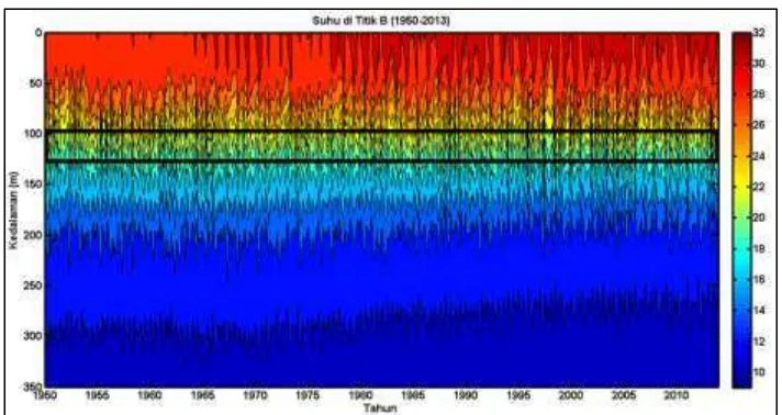
Figure 3 The sea temperature condition in the year of 1950 – 2013 at the point of B. Figure 3 shows the profile T = 22oC isotherm depth at point B in 1950 - 2013. It is located in a depth of 80-130 m. Isotherm depth of T = 22oC changed seasonally (Figure 3). The change distribution of T = 22oC isotherm depth at point B tends to remain in space (depth). Based on table 2, the condition of the shallowest isotherm T = 22oC was in February, when the southwest monsoon. Based Atsari (2013), SSHA in west of Sumatra was still decreasing in February, it indicates that the condition of the thermocline was shallowing. While the condition of the deepest isotherm T = 22oC in November, which is going on second transitional season.
In Figures 3 to 6, the depth of 22oC isotherm shown in the black box. Figure 4 shows the T = 22oC isotherm depth at point of F, and clearly it has the depth range of 100 m. The position of point F located on Lombok strait, which has an important role in a stream passing through the waterway, likely the Indonesian Troughflow (ITF). It shows that the variation T = 22oC isotherm depth is regarded as midthermocline dependent on climatic factors.
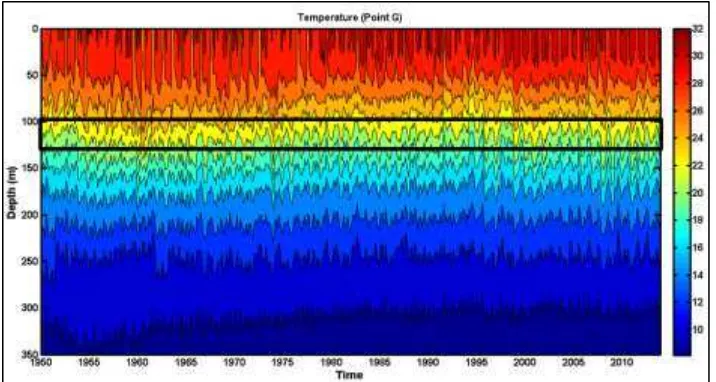
Figure 5 The sea temperature condition in the year of 1950 – 2013 at the point of G. Figures 5 and 6 show display T = 22oC isotherm depth at point G and H. The depth interval has a range of between 90-140 m (50 m) (Table 1). The position of point G and H is situated in the lesser Sunda Island, specifically in 120oLS and 124oLS.
Figure 6 The sea temperature condition in the year of 1950 – 2013 at the point of H. The point of F is located in the southern of Java. Based on Figure 4, the T = 22oC isotherm depth at the point of F has a range of 50-140 m. Based on Table 2, T = 22oC isotherm depth reaches the shallowest point in July, which was going the summer monsoon. Based on Atsari (2013), the summer monsoon has been occurring in June, and it caused the Indonesian sea level was decreasing. Simultaneously, the thermocline was shallowing because of that.
Figures 5 and 6 show the profile of T = 22oC isotherm depth at point G and point H. Point
isotherm depth at point G and H are in the depths of 90-140 m. Based on table 2, T = 22oC isotherm at point G and H have the shallowest condition in August and July, while the T = 22oC isotherm depth was deepening in December.
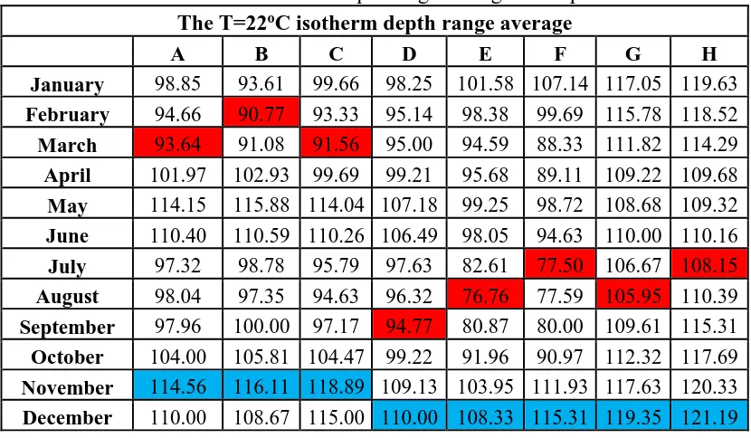
Table 1 The T=22oC isotherm depth range at the point of A-H The T=22oC isotherm depth range (m)
Point
A B C D E F G H
80 – 120 80 - 130 70 - 130 80 - 130 60 - 120 40 - 140 90 - 140 90 - 140
Table 2 The T=22oC isotherm depth range average at the point of A-H The T=22oC isotherm depth range average
A B C D E F G H
January 98.85 93.61 99.66 98.25 101.58 107.14 117.05 119.63 February 94.66 90.77 93.33 95.14 98.38 99.69 115.78 118.52 March 93.64 91.08 91.56 95.00 94.59 88.33 111.82 114.29 April 101.97 102.93 99.69 99.21 95.68 89.11 109.22 109.68 May 114.15 115.88 114.04 107.18 99.25 98.72 108.68 109.32 June 110.40 110.59 110.26 106.49 98.05 94.63 110.00 110.16 July 97.32 98.78 95.79 97.63 82.61 77.50 106.67 108.15 August 98.04 97.35 94.63 96.32 76.76 77.59 105.95 110.39 September 97.96 100.00 97.17 94.77 80.87 80.00 109.61 115.31 October 104.00 105.81 104.47 99.22 91.96 90.97 112.32 117.69 November 114.56 116.11 118.89 109.13 103.95 111.93 117.63 120.33 December 110.00 108.67 115.00 110.00 108.33 115.31 119.35 121.19
Table 2 shows the monthly average of T = 22oC isotherm depth at point of A to H. The depth of T=22oC isotherm variation change in spatial and time, shown in Table 2. When the summer monsoon, thermocline is moving westward and having the shallowest conditions, i.e. in July-September. Meanwhile, when the winter monsoon, the thermocline is reaching the deepest conditions than usual, it was occurring in in November and December for each point. When the first transitional period (March to May), the T=22oC
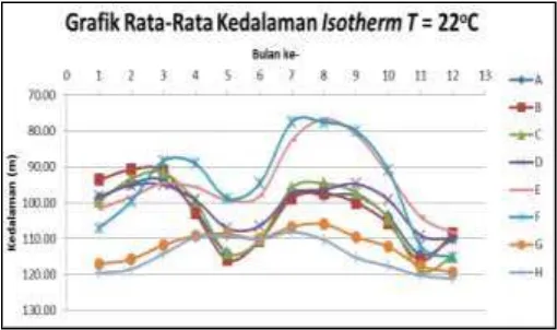
Figure 7 The graph of T=22oC isotherm depth at the point of A to H
Figure 7 shows the change of the T=22oC isotherm depth as the monthly average at the point of A to H. From that graph, could be seen that the point E and F has a large depth variation, as large as 60 to 100 m.
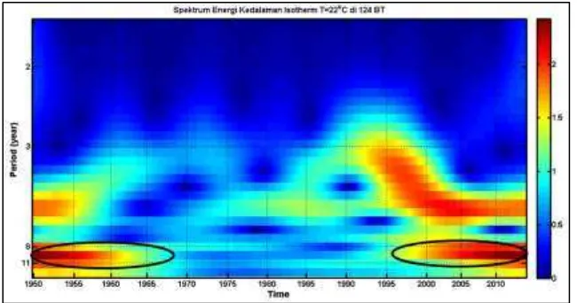
4. The Energy Spectrum of T=22oC Isotherm Depth
After T = 22oC isotherm depth was determined, the next method was used to observe energy spectrum of the depth of the isotherm T = 22oC using s-transform for each point. Figure 8 shows the energy spectrum of T = 22oC isotherm depth at point B and it has a
period of eight yearly.
Figure 8 The energy spectrum of T = 22oC isotherm depth by using the S-transform at
the point of B.
Figure 9 The energy spectrum of T = 22oC isotherm depth by using the S-transform at
the point of F.
Figure 10 The energy spectrum of T = 22oC isotherm depth by using the S-transform at the point of G.
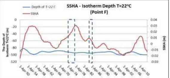
Figure 12 The relation between SSHA and T=22oC isotherm depth at the point of F. the
dashes box as the time of the Kelvin wave propagation.
When the SSHA was increasing, the T=22oC isotherm depth was decreasing. Likewise, when SSHA has decreased, midthermocline conditions have increased. Based on the Figures 12 and 13, the condition of SSHA and T=22oC isotherm depth at the time of the incident wave Kelvin can be observed, i.e. in the year 1974-1976 and 1985-1986 (Khoirunnisa et al, 2016). At the point of B, F, G, and H, when the Kelvin wave was propagating can caused the SSHA conditions are going to rise and midthermocline were deepening, likely in the year of 1974 - 1976.
Figure 13 The relation between SSHA and T=22oC isotherm depth at the point of H. the dashes box as the time of the Kelvin wave propagation.
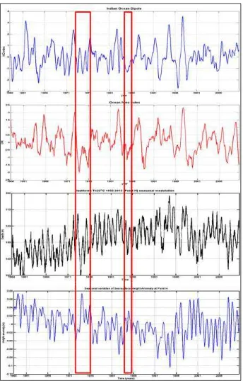
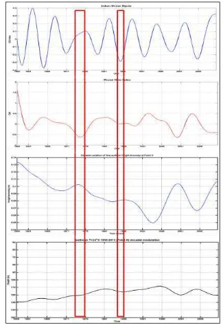
Figures 14 and 15 show the relation between the IOD, ONI, SSHA, and T=22oC isotherm depth condition in seasonal and decadal variations. The red boxes indicate the time of the decadal Kelvin wave propagation, and it shows that the condition of the SSHA and T=22oC isotherm depth have the negative correlation. Figure 15 shows the decadal variation of the IOD, ONI, SSHA, and T=22oC isotherm depth and also the decadal Kelvin wave propagation. When the decadal Kelvin wave was propagating in the year of 1974 – 1976, the decadal modulation of IOD had increasing, meanwhile the ONI had decreasing. At the same time, the positive IOD co-occurred with the El Nino, it makes the SSHA increased than normal condition and the midthermocline is going to decrease. It proved the influence of decadal Kelvin wave into the decadal variation thermocline depth.
According to Treanary and Han (2013), the correlation between SSHA and thermocline depth variability is 0.84. It more strength the hypothesis that the decadal Kelvin waves exist in the western of coast Sumatra and Southern coast of Java and also it influenced the thermocline depth.
Figure 15 The condition of IOD, ONI, T=22oC isotherm depth, and SSHA during the Kelvin wave occurrence (red boxes) by seven years lowpass filter.
5. Wavelet coherence between SSHA and T=22oC Isotherm Depth
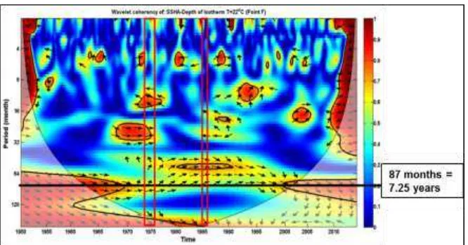
There was the Kelvin wave propagation in along the west of Sumatra and Southern of Java with a period of 7.25 to 7.3 years (Khoirunnisa et al, 2017). This is consistent with the results of wavelet coherency of the points of A, B, C, D, E, and F which have the coherence with a period of 7.25 years between SSHA and 22oC isotherm depth (Figures 20 and 21). In Figures 20 to 23, there are two red boxes indicating time of occurrence Kelvin waves, which in 1974-1976 and 1985 - 1986. Figure 21 shows the coherence with a period of 7.25 years at point of F in a Kelvin wave propagation time, such as during 1974 - 1976. It shows the influence of the decadal Kelvin wave to the T=22oC isotherm depth by decadal period.
Figure 16 The wavelet coherence between SSHA and T=22oC isotherm depth at the
point of B. The red box shows the occurrence of Kelvin wave in the year of 1974 to 1976 and 1985 to 1986.
Figure 17 The wavelet coherence between SSHA and T=22oC isotherm depth at the point of F. The red box shows the occurrence of Kelvin wave in the year of 1974 to 1976
and 1985 to 1986.
Figure 18 The wavelet coherence between SSHA and T=22oC isotherm depth at the point of G. The red box shows the occurrence of Kelvin wave in the year of 1974 to 1976
and 1985 to 1986.
Figure 19 The wavelet coherence between SSHA and T=22oC isotherm depth at the point of H. The red box shows the occurrence of Kelvin wave in the year of 1974 to 1976
and 1985 to 1986.
Conclusion
Reference:
Atsari, R. R. 2013. Studi Variabilitas Tinggi Muka Air Laut di Perairan Selatan Selatan Indonesia. Bachelor thesis. Retrieved from Department of Oceanography, Bandung Institute of Technology.
Bray, N. A., S. Hautala, J. Chong and J. Pariwono. 1996. Large-scale sea level, thermocline, and wind variations in the Indonesian troughflow region. Journal of Geophysical Research, 101:12239-12254.
Clarke, C. O., P. J. Webster, dan J. E. Cole. 2003. Interdecadal Variability of the Relationship between the Indian Ocean Zonal Mode and East African Coastal Rainfall Anomalies. Journal of Climate, 16:548 – 554.
Cooley, J. W dan J. W. Tukey. 1965. An algorithm for the machine calculation of complex Fourier series. Mathematics of Computation, 19:297–301.
Februarianto, M. 2013. Pengaruh Gaya Lokal dan Non Lokal Terhadap Variabilitas Kekuatan Upwelling di Laut Banda. Tugas Sarjana. Program Studi Oseanografi. FITB-ITB. Bandung.
Grinsted, A., J. C. Moore, dan S. Jevrejeva. 2004. Application of the Cross Wavelet Transform and Wavelet Coherence to Geophysical Time Series. Nonlinear Processes in Geophysics, 11: 561 – 566.
Han, W., G. A. Meehl, and A. Hu. 2006. Interpretation of tropicalthermocline cooling in the Indian and Pacific oceans during recent decades,Geophys. Res. Lett., 33, L23615, doi:10.1029/2006GL027982.
Han, W., J. W. Wang, dan J. Weiss. 2008. Interannual Variability and Decadal Change of Themocline Depth and Upper Ocean Heat Content in the Indian Ocean. Department of Atmospheric and Oceanic Sciences (ATOC). USA.
Iskandar, I., W. Mardiansyah, Y. Masumoto, dan T. Yamagata. 2005. Intraseasonal Kelvin Waves along the Southern Coast of Sumatra and Java. Journal of Geophysical Research, 110: C04013.
Khoirunnisa, H. 2015. Variabilitas Interannual dan Dekadal Anomali Tinggi Muka Laut di Perairan Selatan Jawa. Bachelor thesis. Retrieved from Department of Oceanography, Bandung Institute of Technology.
Mantua, N. J., dan S. R. Hare. 2001. The Pacific Decadal Oscillation. Journal of Oceanography, 58: 35 – 44.
Mahongo, S., M. Nguli, and J. Francis. 2014. Inter-annual and Decadal Oscillations of Sea Level in the Western Indian Ocean. Geophysical Research Abstracts, 16: EGU2014-6153-2.
Ningsih, N. S., S. Hadi, I. Sofian, Kunarso, dan F. Hanifah. 2012. Kajian Dampak Perubahan Iklim Terhadap Dinamika Upwelling Sebagai Dasar Untuk Memperkirakan Pola Migrasi Ikan Tuna di Perairan Selatan Jawa – Nusa Tenggara Barat dengan Menggunakan Model Transpor Temperatur Laut. Laporan Riset dan Inovasi KK. Institut Teknologi Bandung. Bandung.
Park, W. S., dan I. S. Oh. 2000. Interannual and Interdecadal Variations of Sea Surface Temperature in the East Asian Marginal Seas. Progress in Oceanography, 47: 191 – 204. Qian, W., H. Hu, Y. Deng, dan J. Tian. 2001. Signals of Interannual and Interdecadal Variability of Air-Sea Interaction in the Basin-Wide Indian Ocean. Atmosphere – Ocean, 40: 293 – 311.
Roisin, C.B. dan M. B. Jean. 2008. Introduction to Geophysical Fluid Dynamics. Academic Press.
Saji, N. H., B. N. Goswami, P. N. Vinayachandran, dan T. Yamagata. 1999. A Dipole Mode in the Tropical Indian Ocean. Nature, 401: 360 – 363.
Schott, F. A., S. P. Xie, J. P. McCreary Jr. 2009. Indian Ocean Circulation and Climate Variability. Reviews of Geophysics, 47: RG1002.
Sprintall J., A. L. Gordon, R. Murtugudde, dan R. D. Susanto. 2000. A Semiannual Indian Ocean forced Kelvin Wave Observed in the Indonesian Seas in May 1997. Journal of Geophysical Research, 105: 17,217 – 17,230.
Stewart, R. H. 2008. Introduction To Physical Oceanography. Department of Oceanography Texas A & M University.
Susanto, D. R., A. L. Gordon, dan Q. Zheng. 2001. Upwelling along the Coasts of Java and Sumatra and its Relation to ENSO. Geophysical Research Letters, 28: 1599 – 1602.
Syamsudin, F., A. Kaneko, dan D. B. Haidvogel. 2004. Numerical and observational estimates of Indian Ocean Kelvin Wave intrusion into Lombok Strait. Geophysical Research Letters, 31: L24307.
Tomczak, M., dan J. S. Godfrey. 2001. Regional Oceanography: An Introduction. Permagon. Tarrytown. New York.
Trenary, L.L. and Han, W., 2013. Local and remote forcing of decadal sea level and thermocline depth variability in the South Indian Ocean. Journal of Geophysical Research:
Oceans, 118(1), pp.381-398.
Wang, Y. H. 2010. The Tutorial: S-Transform. National Taiwan University. ROC.
Xie, S. P., H. Annamalai, F. A. Schott, J. P. McCreary Jr. 2001. Structure and Mechanisms of South Indian Ocean Climate Variability. Journal of Climate, 15: 864 – 878.
Yuan, Y., C. L. J. Chan, Z. Wen, dan L. Chongyin. 2008. Decadal and Interannual Variability of the Indian Ocean Dipole. Advances in Atmospheric Sciences, 25: 856 – 866.