WORKING PAPER 49-2020
LEADING INDICATORS OF POVERTY IN INDONESIA:
APPLICATION IN
THE SHORT-TERM OUTLOOK
Dhanie Nugroho Priadi Asmanto Ardi Adji
JULY 2020
Taufik Hidayat
2
This working paper was prepared for the National Team for the Acceleration of Poverty Reduction (Tim Nasional Percepatan Penanggulangan Kemiskinan: TNP2K). It presents the findings of our ongoing work to encourage discussion and exchange of ideas in the areas of poverty, social protection, and development.
The findings, interpretations, and conclusions in this working paper constitute the opinion of the authors and do not reflect the opinion of the Government of Indonesia or the Government of Australia. Support for this publication is given by the Government of Australia through the MAHKOTA Program.
Copying, dissemination, and transmission of this work for non-commercial purposes are allowed.
Suggested citation: Nugroho, D., P. Asmanto, and A. Adji. 2020. “Leading Indicators of Poverty in Indonesia: Application in the Short-Term Outlook.” Working Paper 49/2020.
Jakarta, Indonesia: National Team for the Acceleration of Poverty Reduction.
To request a copy of the report or request further information, please contact TNP2K ([email protected]). This working paper is also available on the TNP2K website (www.tnp2k.go.id).
NATIONAL TEAM FOR THE ACCELERATION OF POVERTY REDUCTION Office of the Vice President Secretariat
Jl. Kebon Sirih Raya No.14, Central Jakarta, 10110
TNP2K Working Paper 49-2020 July 2020
LEADING INDICATORS OF POVERTY IN INDONESIA: APPLICATION
IN THE SHORT-TERM OUTLOOK
Dhanie Nugroho Priadi Asmanto
Ardi Adji
4
Abstract
Development indicators operate very dynamically in line with the government’s program and policy response.
The government, therefore, needs an estimate of the poverty rate for a specific period in line with the development of its constituent indicators. The rate is required by the government to ensure the implemented policy can achieve the target according to the plan. Given the available indicators, these leading indicators are more dynamic than the poverty line so they need to be monitored earlier to estimate the poverty line in a specific period.
This study varies from previous similar studies, where the poverty projection was made against all poverty indicators. In addition, an analysis was conducted at the national and regional (provincial, rural, and urban) levels in line with the indicators in the official publication of Statistics Indonesia (Badan Pusat Statistik: BPS). This study measures the impact of price increases on expenditure per capita, so the impact on the poverty line can be measured by observing changes in expenditure per capita. This study also formulates a method that can be replicated by policy makers by using inflation rate, economic growth, and population estimate for a specific period. This study concludes that it is very possible to apply the total inflation rate as a leading indicator to project the poverty rate if the government and other stakeholders require an alternative calculation before official figures become available. Nevertheless, the use of inflation in projecting the poverty rate is clearer than economic growth.
Keywords: Inflation, Economic Growth, Poverty Line
6
List of Content
Overview... ... 8
Introduction ... 8
Calculation of Poverty Rate in Indonesia ... 9
Poverty Indicators ...11
Poverty Level ...11
Number of Poor ...11
Poverty Gap ...11
Poverty Severity ...12
Leading Indicators of Poverty Rate ...13
Inflation Rate ...13
Economic Growth ...14
Population Growth ...15
Poverty Rate Calculation Components...16
Expenditure per Capita ...16
Inflation ...16
Temporary Poverty Line ...17
Poverty Line ...17
Food Group ...18
Non-Food Group ...18
Population Number ...19
Assumptions, Data, and Methodology ...20
Projection Assumptions and Scenarios ...20
Data... ...20
National Socioeconomic Survey (SUSENAS) ...20
CPI ...21
Economic Growth ...21
Population Growth ...21
Methodology ...21
Modification to Expenditure per Capita ...21
Modification to Poverty Line ...22
Outcomes and Discussion ...22
Consumption Growth at the Household Level ...25
Poverty Indicator Overview... ...26
Conclusions and Recommendations ...27
Bibliography ...29
Appendix... ...30
8
Overview
Introduction
Poverty alleviation constitutes one of the main policy priorities of the Government of Indonesia. This is in line with the commitment to achieve the first objective in the Sustainable Development Goals (SDGs)–namely eradicating poverty. The availability of an accurate poverty rate in each region that can be compared at the national level constitutes an absolute pre-condition to developing a poverty alleviation policy.
The poverty rate has several functions in national development. The first function is to provide a basis for development of a national development policy and plan, including a policy and plan to improve people’s welfare and sectoral development. The second function, used in targeting, is based on geographical location and individuals and households that are the target of development programs. The third function is to determine the allocation of poverty alleviation and welfare improvement programs. Fourthly, to serve as a monitoring and evaluation indicator of development programs including achievement of the National Medium- and Long- Term Development Plans (Rencana Pembangunan Jangka Menengah Nasional: RPJMN/Rencana Pembangunan Jangka Panjang Nasional: RPJPN) and the Sustainable Development Goals (SDGs). The last function is as an instrument to measure the performance of central and regional governments.
Development indicators operate very dynamically in line with the government’s program and policy response.
The government, therefore, needs an estimate of the poverty rate for a specific period that aligns with the development of its constituent indicators. The poverty rate is required by the government to ensure the implemented policy can achieve the target according to the plan. The macro indicator dynamics at least have an impact on poverty rate, both directly and indirectly.
There are several leading indicators that can be used as a benchmark for estimating the poverty rate: inflation rate, economic growth, and population growth. Given the available indicators, these leading indicators are more dynamic than the poverty line so they need to be monitored earlier to estimate the poverty line in a specific period.
Economic growth describes the increase in aggregate income capacity. Aggregate economic growth is a reflection of household consumption growth in a specific period. In the calculation of poverty rate, the main component is household consumption per capita. The scale of the rate can more or less be estimated through the economic growth indicator. In addition, the economic growth rate is generally published earlier than the poverty rate, thus allowing it to be used as a leading indicator in estimating the poverty rate.
Inflation describes changes in the price of people’s needs from time to time. The price change in important commodities, therefore, needs to be taken into account by policy makers. On the other hand, a specific basket of goods has a direct impact on calculation of the poverty rate, especially 52 food commodities and 36 non-
food commodities. This component further influences the size of the poverty line and poverty rate during a specific period.
In addition, population growth becomes one of the three indicators determining the calculation of poverty rate. Population growth basically uses the result of population projection calculations usually provided by BPS. This rate determines the calculation of poverty rate, especially in the indicator for the number of poor.
The government does not yet have the standard tools or format to estimate the poverty rate for a specific period in the future, although the leading indicator is available earlier than the poverty rate. This condition, therefore, serves as the basis for the importance of developing a poverty projection model that can be used as a means to detect achievements in poverty alleviation and the steps needed to anticipate an increase in the poverty rate.
This poverty projection study is different to previously conducted studies. Firstly, in this study, the poverty projection was made on all poverty indicators. The indicators produced include: poverty line, poverty level, number of poor people, poverty gap, poverty severity, and expenditure per capita which are the main instruments of calculation. The analysis was conducted at the national and regional (provincial, rural, and urban) levels in line with the indicators in official BPS publications. Second, this study measures the impact of price increases on expenditure per capita so the impact on the poverty line can be measured by observing changes in expenditure per capita. Third, this study also formulates a method that can be replicated by policy makers by using inflation rate, economic growth, and an estimate of population numbers in a specific period .
Calculation of Poverty Rate in Indonesia
In calculating poverty in Indonesia, BPS uses a household capability concept to meet basic needs–known as the “basic needs approach”. The “basic needs” refer to the fundamental requirements for fulfilling the minimum needs for a decent life, namely fulfilling the minimum food and non-food needs. With this approach, the measurement of poverty is an inability in terms of expenditure or income to provide for a minimum decent life based on a minimum number of food commodities (food basket) to fulfil calorie needs, together with a number of non-food expenditures (non-food basket). Insufficient income or expenditure or revenue for a minimum decent life is a monetary or poverty line approach or poverty line, namely the value of expenditure to fulfil minimum basic needs in rupiah (monetary approach). The poor population is, therefore, the population having an average expenditure per capita per month below the poverty line.
The poverty line is the sum of the Food Poverty Line (Garis Kemiskinan Makanan: GKM) and Non-Food Poverty Line (Garis Kemiskinan Bukan Makanan: GKBM). GKM constitutes the expenditure value of minimum food needs equal to 2,100 calories per capita per day. The package of basic food commodity needs is represented by 52 types of commodity (grains, tubers, fish, meat, eggs and milk, vegetables, legumes, fruits, oil, and fats). The GKBM constitutes the package of basic non-food needs to meet the minimum need for housing, clothing, education, and health. It includes 51 types of commodity in urban areas and 47 types of commodity in rural areas.
The focus of this study defines poverty as a household’s or individual’s inability to meet the minimum needs for a decent living standard. Nevertheless, poverty in general can have a broad meaning. The definition of minimum decent need and the method of measuring it determines the magnitude of the poverty line and, therefore, of the poverty rate.
10
BPS is the institution authorised by the government to calculate and map the official rate of poverty in Indonesia from time to time. BPS has calculated poverty since the early 1980s and published it officially in 1984. The publication covers the poverty rate for the period 1976-1981. Since then, every three years, BPS has calculated the number and percentage of the poor population in Indonesia together with available household consumption data collected from the National Socioeconomic Survey (SUSENAS). Since 2002, the poverty calculation is undertaken annually through the household consumption module survey of SUSENAS.
Poverty Level
The Head Count Index (HCI-P0) is the percentage of the population with expenditure per capita below the poverty line. The poor are those below the poverty line. The poverty level is calculated using the following formula:
(1)
Where is 0; is the poverty line; is the average expenditure per capita in a month for those below the poverty line (i=1, 2, 3, ...., q), < z; is the population number below the poverty line; and is the population number.
Number of Poor
The poor population is the number of people living below the poverty line during a specific period. In accordance with the previous formulation, the poor population is calculated every six months, namely in March and September.
For the government, the poor population number is the development target which needs to be lowered every year.
Various government programs and policies are directed to achieving a poor population number in accordance with the target in the development plan. Several programs are aimed at reducing the expenditure burden through the social protection program. In addition, to increase household incomes, a similar policy is also applied, but in a different dimension, such as the people’s business credit program and village fund.
Poverty Gap
The Poverty Gap Index-P1 is the average measure of expenditure gap between each poor person and the poverty line. The higher the index value, the further the average person’s expenditure is from the poverty line:
(2)
Where is 1; is the poverty line; is the average expenditure per capita in a month for those below the poverty line (i=1, 2, 3, ...., q), < z; is the population number below the poverty line; and n is the population number.
Poverty Indicators
12
In general, this index is useful for determining the cost of poverty eradication by creating an ideal transfer target for the poor population by assuming perfect targeting–without any leakages or program obstacles.
The lower the poverty gap value, the greater the economic potential for poverty eradication funds based on identifying the characteristics of the poor population and targeting assistance and programs. A fall in the value of the poverty gap index indicates that the average expenditure of the poor tends to become closer to the poverty line and the expenditure inequity of the poor also narrows.
Poverty Severity
The Poverty Severity Index-P2 gives an illustration of expenditure spread across the poor population. The formula used to determine the index is:
(3)
Where is 2; is the poverty line; is the average expenditure per capita in a month for those below the poverty line (i=1, 2, 3, ...., q), < z; is the population number below the poverty line; and ais the population number.
In general, the higher the index value, the higher the expenditure imbalance among the poor population.
This index is useful for providing complementary information on poverty incidence. For example, there may be cases where some groups of poor have a high poverty incidence but their poverty gap is low, while other population groups have a low poverty incidence but a high poverty gap for the poor population.
Inflation Rate
The inflation rate is generally published by BPS through the Statistics Official News (Berita Resmi Statistik: BRS) in the first week after the end of the reporting month. For example, the inflation rate of March is published in the first week of April. The inflation rate rolled out in this publication includes monthly, annual, and current year inflation. Meanwhile, the poverty rate and its indicators are published in the first week after the quarterly survey. The inflation rate in this study has, therefore, been established as a leading indicator of the poverty rate. Establishing the inflation rate as a leading indicator is based on the impact of inflation on the poverty rate and being the number published before the poverty rate.
Several studies related to the impact of inflation on the poverty rate and household expenditure have been conducted. To measure the impact of price changes on public welfare, Son and Kakwani (2008) and Son (2008) assume that expenditure per capita is the function of price ( ) and utility ( ) reflecting living needs.
(4)
The formula indicates that the expenditure per capita depends on the efforts of these individuals to meet their expected living needs at a specific price. A price change, like an increase in to *, forces these individuals to compensate the increase in price in order to achieve the same utility level. This assumption serves as the basis for these two researchers to measure the real change of expenditure per capita as a consequence of a price increase, which is then expressed in the following equation:
(5)
By applying the Taylor expansion rule, the following equation is obtained.
(6)
The above equation assumes that there is no substitution effect of goods when there is a price increase in the goods. From a relative increase in commodity , the impact of a fall in expenditure per capita can be calculated in accordance with the price elasticity of commodity , as set out in the following equation:
(7)
The equation above indicates that there is an increase in the price of commodity by 1 per cent causing a decrease in welfare of the individual by a percentage proportionate to the expenditure per capita of the
Leading Indicators of Poverty Rate
14
At the population level, the impact of a price increase has the same principle as that on the individual’s expenditure per capita. This calculation concept commences by changing the concept of individual expenditure per capita into the concept of expenditure per capita at the population level . Where is the density function of . To obtain the price elasticity of the population’s expenditure per capita, the following equation is lowered against price, thus the following elasticity formula is obtained:
(8)
The average expenditure per capita of the entire population for commodity is marked as while reflects the total expenditure per capita of the entire population. Meanwhile, is the average proportion of expenditure per capita for commodity . Interpretation of this equation is identical to equation 6, where every 1 per cent increase in commodity will reduce population welfare by %, or equal to the price elasticity of such goods.
Given that changes in commodity prices vary from one commodity to another, the resulting impact between commodities will differ. To capture the impact of a price change of each commodity on a change in welfare level, equation 8 can be composed into the following equation:
(9)
The equation above measures the real change occurring in public welfare as a consequence of a price change in every commodity. This can be seen from the average public welfare in the base (period) year when the price of commodity is . When there is a price increase from to *, the average public welfare also undergoes an increase to *. In a more mathematical manner, every price increase by r per cent will decrease the welfare level by . The impact of a price increase in each commodity on the public welfare is then referred to as the within effect.
Economic Growth
One of the important indicators to identify the economic condition in a country in a specific period is Gross Domestic Product (GDP), based on both the prevailing price and constant price. In general, GDP is basically the amount of additional value generated by all business units in a specific country, or the final value amount of all goods and services produced by all economic units.
GDP based on prevailing price describes the additional value of goods and services calculated using the prevailing price in every year. GDP based on constant price indicates the additional value of the goods and services calculated by using the prevailing price in one specific year as the basis. GDP based on the prevailing price can be used to observe economic structure and movements, while the constant price is used to determine economic growth from year to year.
The regular economic growth rate is published by BPS through BRS during the first week in the second month after the report. For example, economic growth for the first quarter is published in the first week of May.
The economic growth rate reported in this publication includes quarterly and annual economic growth. The poverty rate and its indicators are published in the first week after the three month survey.
The economic growth rate is used in this study as a leading indicator of the poverty rate and is based on the impact of economic growth on poverty rate. It is also published before the poverty rate. For example, the poverty rate for March is published by BPS through BRS in the first week of July while the economic growth rate has already been published in May.
Population Growth
Population growth indicates the annual population increase for a specific period. The method most often used by BPS is the geometrical method, although the population growth rate can also be calculated using the arithmetic or exponential method. In each survey conducted by BPS, population growth is the change in individual weighting, and this also has implications on the calculation of poverty rate.
The population projection has been published by BPS for 2015 until 2045. This rate is available based on age group, gender, and province, for both rural and urban areas. Referring to the publication, it is quite relevant to use population growth as one of the leading indicators in making poverty indicator projections in Indonesia.
16
Expenditure per Capita
Expenditure per capita is the cost incurred for consumption of all household members for a month divided by the number of household members. Data on expenditure can reveal the household consumption pattern in general by using the indicator of proportion of expenditure allocated to food and non-food commodities. The household expenditure composition can be used to assess the economic welfare level of the population–a lower level of total expenditure spent on food is generally an indication of an improved welfare level of the household or individual.
Household expenditure is differentiated based on food and non-food groups. A change in someone’s income will influence a shift in their expenditure pattern. The higher the income, the higher their non-food expenditure.
Expenditure pattern can, therefore, be used as one tool to measure people’s welfare level, where a change in its composition is used as an indicator of a change in welfare level.
Expenditure per capita is the main instrument used for calculation of the poverty rate. A person is included in the poor category if their expenditure per capita is lower than the poverty line. The availability of expenditure per capita, therefore, constitutes the main data source for calculation of the poverty rate and serves as the basis for estimating the national and regional (provincial, urban, and rural) poverty rate estimation.
Inflation
The inflation rate is a change in the Consumer Price Index (CPI). In general, CPI is an economic indicator that provides information on the price of goods and services purchased by consumers. Calculating the CPI is undertaken to record changes in the purchasing price at the consumer level (purchasing cost) of a fixed group of goods and services (fixed basket) that are generally consumed by the community–more commonly referred to as the inflation rate.
CPI is the cost price index of a group of consumer goods, each of which is weighted according to the proportion of public spending on the commodity concerned. CPI measures the price of a group of specific goods such as main foodstuffs, clothing, housing, and miscellaneous goods and services purchased by consumers in a specific period.
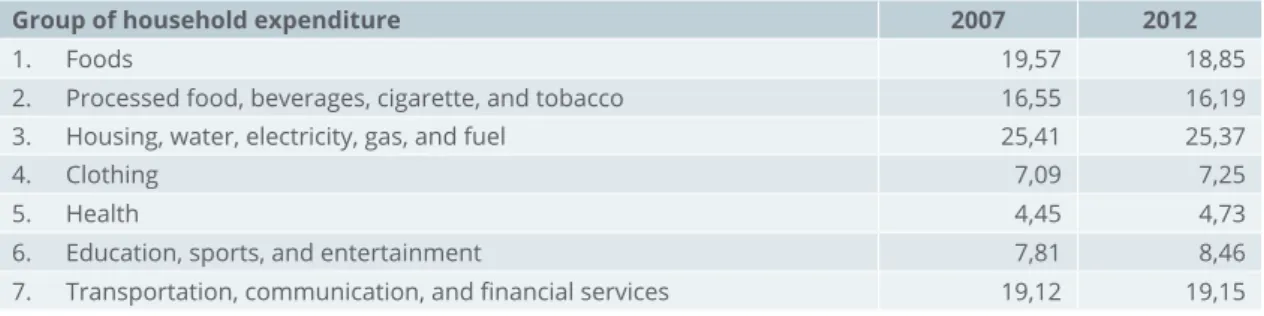
Calculation of the CPI is done by referring to the cost of living survey to determine the type of commodity in the CPI. This survey is conducted once every seven years, with the last survey conducted in 2012. At the moment, CPI records 859 types of commodity classified into seven groups: (i) foodstuffs; (ii) processed food, beverages, cigarettes, and tobacco; (iii) housing, water, electricity, gas, and fuel; (iv) clothing; (v) health; (vi) education, recreation, and sports; and (vii) financial services. The number of recorded commodities has increased in comparison with the CPI based on the Cost of Living Survey 2007 which only recorded 774 commodities. Table 1 shows the change in the weighting composition of seven groups of goods in the calculation of Indonesia’s CPI.
Poverty Rate Calculation Components
Inflation contributes to the calculation of poverty rate–especially in the calculation of the poverty line. Inflation is the inflator of temporary poverty line before it is applied in the reference population. Availability of the inflation rate in each time period is an inseparable component in the calculation of poverty rate in Indonesia.
Table 1 Weight composition of goods 2007 & 2012
Group of household expenditure 2007 2012
1. Foods 19,57 18,85
2. Processed food, beverages, cigarette, and tobacco 16,55 16,19
3. Housing, water, electricity, gas, and fuel 25,41 25,37
4. Clothing 7,09 7,25
5. Health 4,45 4,73
6. Education, sports, and entertainment 7,81 8,46
7. Transportation, communication, and financial services 19,12 19,15
Temporary Poverty Line
The temporary poverty line is defined as the poverty line of the previous period adjusted for general inflation in the CPI. This temporary poverty line is calculated using the following formula:
(10)
Where is the temporary poverty line in period of province and area ; is the poverty line in period t-1 of province and area ; is the inflation in period t of province and area .
Calculating the temporary poverty line is the first step in calculating the poverty rate. The rate serves as the basis for determining reference population that is the benchmark for calculating the poverty line. The reference population is the 20 per cent of the population above the temporary poverty line. Based on this reference population, the GKM and GKBM are subsequently calculated.
The reference population serves as a method for calculating the poverty line. This reference population is defined as the population having expenditure per capita between the temporary poverty line and its maximum reference, namely 20 per cent above the temporary poverty line:
(11)
Where is the temporary poverty line and is expenditure per capita between the temporary poverty line and its cap.
Poverty Line
Calculating the poverty line in Indonesia is conducted by following the cost of basic needs (CBN) method. This method uses a consumption sufficiency approach equal to 2,100 calories per individual per day. There are two expenditure components used to calculate the total poverty line, namely the food consumption group poverty line and non-food consumption group poverty line. There are 52 types of food commodity used to calculate the GKBM, while the non-food group poverty line is calculated based on 36 types of goods.
(12)
18
Where Z is the total poverty line, dan are the food and non-food poverty lines respectively. Furthermore, the poverty line is calculated based on location–namely based on province and region (urban and rural).
Food Group
The consumption value per capita for 52 types of food commodity is used in calculating the poverty line for the food group. This consumption value is also calculated based on location, in this case based on province j and area type a (urban or rural). The formula for calculating individual consumption value per location per area is in the following mathematical equation:
(13)
Where is the poverty line for the food group (m) in province and area . The average price of commodity in province and area is marked as , while is the average amount of the same commodity in this location consumed by an individual. Meanwhile, indicates the average consumption value consumed by an individual in province and area . Furthermore, this consumption value is the equivalent of the daily minimum calorie need of 2,100 calories. This is calculated by applying the following formula:
(14)
Where is the average implicit price per calorie in area and province for the food group which has been equated to 2,100 calories. Notation is the calorie value for every commodity in area and province .
Non-Food Group
Unlike the calculation for the food group poverty line, the poverty line for the non-food group is calculated by applying ratio between commodity and total non-food consumption in each (urban and rural) area. This is done due to a difference in data structure, where the non-food group does not contain any calories as in the foodstuffs group. The non-food group consumption ratio used refers to the basic need commodity package survey conducted in 2004. This ratio value is multiplied by the consumption value per non-food commodity type in every area by following the formula:
(15)
Where is the non-food poverty line in province and area . Meanwhile and are respectively the consumption ratio of commodity in non-food group in area to total non-food consumption in area and the consumption value of commodity in province .
Population Number
The availability of population data has at least several benefits. The data is required to estimate various population parameters down to a specific administrative region. The data is also used to collect population information that can be used/utilised to compose the basis for population data.
The population number is defined by BPS as the number of people who have a permanent residence, and whose census details are collected where they usually reside. People who are travelling for six months or more, or who have been in a residence for six months or more, are counted where they reside at the time of census.
In accordance with this definition, the population of a region consists of five groups. The first one is a person residing in a region permanently or who has already been there for six months or more. The second one is a person residing in a region for less than six months but intending to permanently reside there. The third one is a person who is travelling to another region for less than six months and does not intend to settle permanently in the destination region. The fourth one is a person residing in a region by contracting/
renting/staying in a boarding house, for work or school and might move again for various reasons. The fifth one is a member of the Indonesian diplomatic corps (ambassador, consul, and other Indonesian representatives having the status of diplomat) and his/her family members residing overseas.
In addition, there are five categories of people who are not included as residents of a region. The first one is a guest who is visiting for less than six months and who does not intend to reside there permanently. The second one is a person who is travelling to another region for six months or more. The third one is a person who has moved and intends to reside permanently in the destination region although he/she has not left this residence for six months. The fourth one is a person who has resided in another region by contracting/renting/staying in a boarding house, although during holidays he/she returns (visits) to the house of his/her family or parents. The last one is a member of the diplomatic corps (ambassador, consul, and other representatives having the status of diplomat) of a foreign country and his/her family members residing in Indonesia.
In relation to the calculation of poverty rate, data on population number is required to calculate the proportion of the population living below the poverty line. The calculation subsequently determines the size of the population living below the poverty line–what is commonly referred to as the poverty rate.
20
Projection Assumptions and Scenarios
The assumptions used determine the simulation result in each projection. Furthermore, the assumptions are developed as the basis for setting scenarios. In short, there are two large groups in the assumptions used to calculate the poverty rate projection.
The first assumption is permanent and is not directly counted. This group consists of: (i) population growth using the rate in the 2015-2045 Population Projection published by BPS; and (ii) the quantity of goods consumed by households in a permanent condition. Population growth indirectly contributes to the calculation of poverty rate, where the size of population growth determines the number of poor in a specific area. Population growth is, therefore, one of the assumptions in this study, with the rate positioned as a constant indicator referring to the outcome of the 2015-2045 Population Projection.
The second group consists of variable assumptions–namely assumptions based on leading indicators that directly influence consumption and the price level of goods and services. These assumptions are among others:
(i) price growth (inflation); and (ii) economic growth. The second assumption of this indicator is a leading indicator and the real rate is published by BPS before the poverty rate is published. In general, the economic growth rate is published two months before the poverty rate is published, while the inflation rate for the same period as the poverty rate is published three months before the poverty rate.
Data
National Socioeconomic Survey (SUSENAS)
This study uses the data published by BPS, namely SUSENAS and CPI. SUSENAS are survey data that record household consumption expenditures and demographic data on members of these households. BPS divides SUSENAS into two data groups (modules), namely individual modules that measure individual demographic characteristics including population demography, education, health, and information related to housing and household assets. The second module measures household expenditures for both food group consumption and non-food group consumption.
The number of samples collected in this survey is 300,000 household respondents spread across 34 provinces and 511 regencies/cities in Indonesia. This study specifically uses the consumption module of SUSENAS that measures household consumption for 358 types of goods, which can be divided into 236 food groups and 122 non-food groups. SUSENAS data is sourced from BPS dissemination and represents the same data set as the one used in the calculation of poverty rate.
Assumptions, Data, and Methodology
CPI
The CPI is one of the indicators used to record price changes occurring at the consumer level for a number of goods and services. The CPI recording method has undergone five evolutions since this method was first adopted by BPS. At the moment, CPI records 859 goods and services generally consumed by the community.
This method refers to the 2012 cost of living survey conducted in 82 cities. These 859 commodities are subsequently divided into seven commodity groups: (i) foodstuffs; (ii) processed food; (iii) housing, water, electricity, gas, and fuel; (iv) clothing; (v) health; (vi) education, recreation, and sport; and (vii) transportation, communication, and financial services. The CPI data originates from BRS that is routinely published by BPS and is earlier than the poverty rate.
Economic Growth
Economic growth is one of the indicators describing the economic condition. This rate represents the level of development success of a region in a specific period. Positive economic growth, therefore, indicates an increase in the production of goods and services that might directly impact on household consumption. In this study, aggregate economic growth and household consumption growth are factors that determine the poverty rate. Economic growth data are sourced from the BRS journal routinely published by BPS and is earlier than the poverty rate.
Population Growth
Population growth depicts the level of population increase per year in a specific period. The method most often used by BPS is the geometrical method although the population growth rate can be calculated using the arithmetic or exponential method. Data on population growth is an output of BPS published in the 2015-2045 Population Projection.
Methodology
The poverty rate prediction in this study follows the concept introduced by Son and Kakwani (2008) and Son (2008) with a number of modifications to adjust for prevailing conditions in Indonesia. To make a prediction, two stages of analysis are undertaken: (i) identifying the magnitude of the impact of price rises on expenditure per capita; and (ii) its impact on the poverty line. By identifying the change occurring in these two components, the poor population after a price increase is defined as individuals having expenditure per capita less than, or equal to, the poverty line.
Modification to Expenditure per Capita
The calculation of the impact of CPI on the level of community welfare level, as expressed in equation 10, is the estimated impact of real price increases on household expenditure. It means that when there is no increase in an individual’s income, the CPI (inflation) causes a real decrease in an individual’s welfare level.
Given that the main objective of this study is predicting expenditure per capita and the poverty rate by using inflation, this study has modified the concept introduced by Son and Kakwani (2008) above. Unlike these two researchers, this study focuses on measuring the impact of a nominal price increase on expenditure per capita and the poverty rate. As an initial stage, this study proposes a hypothesis that a price increase represents direct price elasticity against expenditure per capita. This concept is mathematically expressed as follows:
(16)
22
Where and are the expenditure per capita of periods t and t-1, while and are the CPI occurring in periods and respectively. Equation 16 above may be interpreted that to meet the basic minimum need per day, an individual must increase his/her expenditure per capita to equal the price increase.
Furthermore, the impact of this price increase can be measured on the basis of location–in this case provinces. To make this decomposition, equation 16 above is modified into the following formula:
(17)
This equation shows that national expenditure per capita constitutes the weighted average of a change in expenditure per capita in each province due to a price increase in the province. The weighted proportion used is the proportion of inflation in each province in establishing the national inflation rate . This concept is a method that can measure the between effect of inflation on expenditure per capita.
Like the decomposition of the impact of price increases based on location, the impact of price increases can also be decomposed based on the type of goods group consumed by an individual. There are two goods groups measured, namely the food group and non-food group. To do this, equation 16 can be modified as follows:
(18)
Like equation 17, the equation above sorts out the effects of price increases based on changes occurring by goods group . Where is the average price of goods group in period , while is the average price of goods group in period . Meanwhile, is the weighting between the food group and non-food group used to determine the magnitude of the impact of each goods group on expenditure per capita.
Modification to Poverty Line
Unlike Son and Kakwani (2008) and Son (2008) who measure the impact of price increases on changes in the poverty rate, in the second stage, analysis of the measured impact of price increase is conducted on poverty line. The reason for identifying the impact on poverty line is the poverty line principle that measures the expenditure per capita of the poor population group in meeting their minimum needs.
There are some benefits to be obtained by measuring the impact of price increases on the poverty line.
First, the concept of poverty line that measures the expenditure per capita of a poor individual in meeting his/her daily needs allows this study to measure the inflation occurring in the poor population group. This method is, therefore, able to overcome the bias of CPI as a measure of price increase faced by all individuals.
The importance of identifying the price index faced by the poor is in line with the opinion expressed by Adam and Levell (2014). They are of the opinion that an individual’s consumption pattern at each income distribution level varies from one to another.
Second, the adjustment made to the poverty line makes the conducted analysis dynamic. It means that the poverty line is not considered a fixed line, but changes in line with movements in expenditure per capita. The proposed hypothesis is that a price increase will cause an increase in the poverty line. The impact of price increase on poverty line can be expressed in the following formula.
(19)
Where and Z are the poverty line in periods and . Meanwhile, indicates the scale of the price index faced by the poor population group. If <1, the inflation rate faced by the poor is lower than inflation faced by the non-poor population.
There is one assumption that must be taken into account in this study, namely individual expenditure per capita represents their ability to consume. It means that a price increase for individuals has been compensated by an income increase. With this assumption, if <1 , the poverty line experiences a lower increase than the increase in expenditure per capita. This implies a fall in the poor population in a specific period, given that the ability to meet their daily minimum needs increases at a higher rate than the poverty line. Likewise, when
> 1, the poverty line undergoes a higher increase than expenditure per capita. This can also mean that a price increase faced by the poor is greater compared to the price increase faced by the non-poor population.
Like the impact of a price increase on expenditure per capita, the impact of a price increase on the poverty line can be sorted based on goods group (within effect) and on location (between effect). To identify the impact of a price increase based on location, equation 19 may be assumed as the applicable formula for one province:
(20)
Where is the poverty line in province , while pj is the CPI in province . The national poverty line is the weighted average of provincial poverty line, whereby the weighting used is the proportion of the population of province to total national population. The national poverty line as the weighted average of poverty line of province can be expressed in the following equation.
(21)
Substituting equation 20 into equation 21 obtains a formula to calculate the impact of a price increase occurring in each province in Indonesia on the national poverty line:
(22)
Equation 22 indicates that a price increase in province has a proportionate impact on the change of national poverty line. The greater the weighting of province in the establishment of national poverty line, the greater its influence. Every 1 per cent increase in CPI in province j will, therefore, raise the poverty line by per cent multiplied by the weighting of that province ( ) . Nevertheless, given that CPI in Indonesia is not measured at the area (urban and rural) level, decomposing the impact of a price increase based on location cannot be done at the smaller (area) level and is limited to the provincial level.
The same principle also applies in conducting a review of price increases based on commodity groups on the poverty line. In this study, the commodity groups used are the food group and non-food group. As an initial stage, equation 19 above can be re-expressed in the following equation.
24
The equation above indicates the relationship between a price increase of commodity group with the commodity group poverty line. If it has the same meaning as the poverty line at the provincial level, then every 1 per cent increase in CPI in commodity group will be transformed into an increase in the poverty line by its elasticit . The impact of a price increase in commodity group on the total poverty line can be obtained by calculating the weighted average of the poverty line of each commodity group. This relationship is shown by the following formula:
(24)
Where and are the weighting of commodity group and commodity group respectively on the poverty line. Inserting equation 20 into equation 21 obtains a relationship between the total poverty line and every
price change (CPI) in each commodity group.
(25)
Equation 25 shows the relationship between a price increase of commodity group and the national poverty line. Every price increase (CPI) in commodity group will increase the poverty line by the elasticity percentage multiplied by the weighting of this commodity group ( ).
Consumption Growth at the Household Level
The calculation of inflation in Indonesia follows the modified Laspeyers formula (BPS 2016). As the initial stage, this study conducted a simple analysis to see the impact of a national price increase on welfare level–
represented by expenditure per capita and the poverty line. In this stage, the magnitude of the real rate of inflation faced by the poor population commodity is also estimated (Table 1).
Table 2 National Inflation and Inflation for the Poor (March-September 2018)(%)
Indicator General Inflation
(%) Food Inflation
(%) Non-food
Inflation (%) Assumption
General Inflation 0.94%
Food Inflation 0.35%
Non-food Inflation 1.34%
Economic Growth 5.17%
Household Expenditure Growth 5.03%
Population Growth 0.62%
General
Scenario 1 0.94% 0.94% 0.94%
Scenario 2 0.85% 0.35% 1.34%
Scenario 3 5.17% 5.17% 5.17%
Scenario 4 5.03% 5.03% 5.03%
Poor Group
Scenario 1 0.58% 0.62% 0.51%
Scenario 2 0.44% 0.16% 0.99%
Scenario 3 2.05% 2.31% 1.55%
Scenario 4 2.03% 2.28% 1.55%
Source: BPS and calculation result.
The table above gives an illustration of the application of equations 16 and 19. By following equation 16, the expenditure per capita occurring between March and September 2018 experienced a greater increase compared to the one faced by the poor in all calculation scenarios. The calculation is based on a decomposition conducted in equation 19, where it is known that the actual price increase faced by the poor tends to be lower than general inflation.
Outcomes and Discussion
26
The assumption used in this calculation is that the amount of food and non-food commodity consumption of each household does not change. It is, therefore, assumed that an income increase is also fully expended to cover the price increase of the goods consumed. Inflation and growth reflect national economic growth which is fully reflected in an increase in nominal expenditure constituting the aggregated average of the increase in income obtained by each individual. For that reason, the lower inflation faced by the poor compared to the average national population indicates that the impact faced by the poor from a price increase is smaller than the national population average.
Poverty Indicator Overview
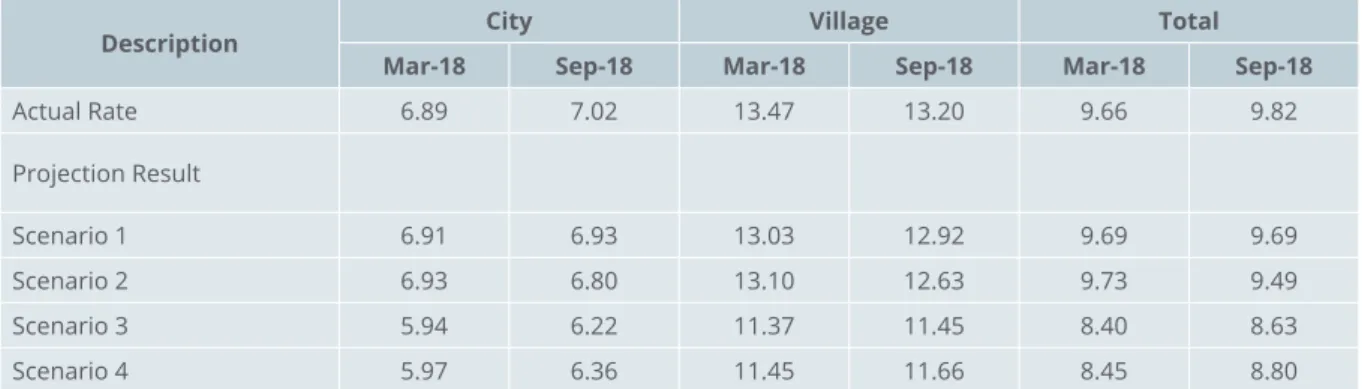
The simulation result indicates an inter-scenario variation although, in general, the poverty line tends to be lower than the actual rate published. As an illustration, in March 2018, the poverty line is about 2 per cent lower than the actual rate while, in September 2018, it is lower by about 3 per cent. In addition, the simulation model used generates a lower deviation in the non-food poverty line group with a difference for all calculation scenarios.
The result of the non-food poverty line projection has a smaller deviation for urban regions than rural regions.
Nevertheless, for the food group poverty line, a smaller deviation in fact is found in rural regions. This can be understood, whereby the calculation of inflation rate is conducted in urban regions consisting of 88 big cities in Indonesia, so rural regions are possibly not fully reflected in the rate calculation. For more details, the rates above can be seen in the attachment.
The estimation simulation of the inter-scenario poverty rate indicates a rate closer to the published rate if the inflation approach is used, rather than the economic growth rate. By using the inflation rate as a leading indicator, the poverty rate in March 2018 is projected with an average deviation below 0.5 per cent. On the other hand, using economic growth as the leading indicator, indicates that the poverty rate projection has a higher deviation, with an average of more than 1 per cent.
Table 3 Future Prospect of Poverty Rate in March and September 2018
Description City Village Total
Mar-18 Sep-18 Mar-18 Sep-18 Mar-18 Sep-18
Actual Rate 6.89 7.02 13.47 13.20 9.66 9.82
Projection Result
Scenario 1 6.91 6.93 13.03 12.92 9.69 9.69
Scenario 2 6.93 6.80 13.10 12.63 9.73 9.49
Scenario 3 5.94 6.22 11.37 11.45 8.40 8.63
Scenario 4 5.97 6.36 11.45 11.66 8.45 8.80
Source: Calculation result based on SUSENAS.
As previously explained, the simulation of future poverty line prospects tends to reflect the actual rate more accurately for urban regions than for rural regions. On average, the deviation of urban regions is below 0.5 per cent if the inflation indicator is used and below 1 per cent if economic growth is used. Nevertheless, the simulation result indicates a greater deviation in the rural regions, for both the inflation and economic growth indicators.
Conclusion
The poverty rate in Indonesia is published by BPS in March and September every year. During this time span, there are published indicators that can be used as leading indicators to predict the poverty rate for the following period. The inflation and economic growth rates are two indicators that can be used as instruments to estimate the poverty rate. It is, however, possible that a number of factors can influence the movements in expenditure per capita and the poverty line, thus eventually influencing the national poverty rate percentage.
This study differs from previous studies that measure the real impact on welfare level, as this study measures more the impact resulting from price increases and economic growth on the poverty line calculated by BPS using a nominal approach. This study measured the effect of price increases and economic growth in 2018 on individual expenditure per capita and the nominal poverty line. The result is used to calculate the poverty rate projection which is then compared to the actual rate published for the same period. This concept is in line with the concept of poverty line measurement in Indonesia which uses expenditure per capita of the reference population to determine the poverty line.
Of the four proposed scenarios, the approach of the first scenario is more accurate than the others. This scenario has the lowest deviation compared to the alternatives, both in urban and rural regions, and for the food and non-food poverty line groups. This result might occur given that the mechanism for calculating the temporary poverty line conducted by BPS uses the total inflation rate as a multiplying factor, instead of using the food or non-food inflation component. In addition, the poverty rate calculated by BPS also does not directly consider economic growth, either in total or by household consumption.
The total inflation rate as a leading indicator can be used to project the poverty rate if the government or other stakeholders require an alternative methodology before the official rate is available. As well as considering the above simulation results, the use of inflation in projecting the poverty rate is clearer compared to economic growth. Changes in the price of goods needed by households directly affects consumption reflected from the cumulative change in prices for each goods group and in total expenditure per capita.
The indicator of economic growth cannot be directly seen in a change of household consumption pattern, especially if the calculation of poverty rate is directly conducted using SUSENAS. In addition, the government and other stakeholders can also identify the consumption pattern of the Indonesian community when there is a price increase in a specific commodity. A good understanding of movements in inflation generally provides an opportunity for stakeholders to determine the policy direction to reduce the poverty rate, at least for the following six-month period.
Conclusions and Recommendations
28
Recommendation
With the urgency to estimate the upcoming poverty rate, while official figure has not been released, utilizing inflation rate as a leading indicator could be beneficial for the government of Indonesia. The estimated figure can capture the household’s purchasing power with the increase in price in a monthly basis, hence providing more updated estimate as compared to quarterly economic growth or official figure in an annual basis.
However, additional consideration is still needed to use this approach:
1. Decomposing poverty rate by considering the inflation rate by type of commodity to fulfil basic needs as the calculation instrument. This measure would benefit the policy makers to identify commodities with significant impact should price increase occurred. Thus, reducing the impact by formulating social assistance program targeting these commodities for specific individuals could be formulated.
2. Regular estimate for poverty rate estimation needs to be made in a monthly basis. This measure can at least improve the understanding of policy makers to apply the appropriate intervention in accordance with movements in the price of basic needs, especially those related to the poverty line commodity components and achieve a poverty rate in accordance with the target.
Bibliography
Prima, R.A, C. Hanum, and R.N. Siregar. 2013. “Consumer Price Indices for the Poor in Indonesia.” Boston:
Boston Institute fo
r Developing Economies.
Deaton, A. 2008. “Price Trends in India and Their Implications for Measuring Poverty.” Economic & Political WEEKLY, Feb 9,2008 43-49.
De Hoyos, R.E. and D. Medvedev. 2009. “Poverty Effects of Higher Food Prices: A Global Perspective.” Policy Research Working Paper 4887. Washington DC: World Bank.
de Janvry, A. and E. Sadoulet. 2008. “Methodological Note: Estimating the Effects of the Food Price Surge on the Welfare of the Poor.” Berkeley: University of California.
Fujii, T. 2011. “Impact of Food Inflation on Poverty in the Philippines.” Working Paper 11-2011. Singapore:
Singapore Management University.
Garner, T.I., D.S. Johnson, and M.F. Kokoski. 1996. “An Experimental Consumer Price Index for the Poor.”
Monthly Labor Review 119 (9): 32-42.
Gibson, J. 2016. “Poverty Measurement: We Know Less than Policy Makers Realize.” Asia & The Pacific Policy Studies 3 (3): 430-442.
Ravallion, M. and D. van de Walle. 1989. “Cost of living differences between urban and rural areas in Indonesia.”
Working Paper Series on Agricultural Policies No. 341. Washington DC: World Bank.
Son, H.H. 2008. “Has Inflation Hurt the Poor? Regional Analysis in the Philippines.” ERD Working Paper Series No. 112. Manila: Asian Development Bank.
Son, H.H. and N. Kakwani. 2008. “Measuring the impact of price changes on poverty.” The Journal of Economic Inequality 7 (4).
Statistics Indonesia. 2009. Pedoman Survei Statistik Harga Konsumen Tahun 2009. Jakarta: Statistics Indonesia.
Adams A. and P. Levell. 2014. Measuring poverty when inflation varies across households. JRF report.
30
Appendix
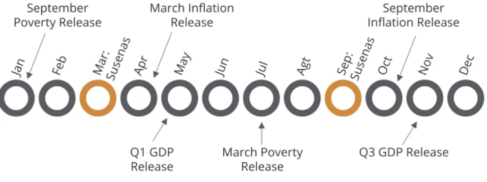
Poverty Rate, Inflation, and Economic Growth Publication Timeline
Jan Feb Mar: Susenas Apr May Jun Jul Agt Sep: Susenas Oct Nov Dec
Q1 GDP
Release March Poverty Release March Inflation
Release September
Poverty Release September
Inflation Release
Q3 GDP Release
Source: BPS and Bank Indonesia
Table 4 Future Calculation Scenario of Poverty Indicator (September 2018 Poverty Release)
Base Assumption Scenario
2 3 4
Constant Variable Group
Quantity of Food/Non-Food Consumption
• • • •
Population Growth
• • • •
Dynamic Variable Group
General Inflation
•
Food/Non-Food Inflation
•
Total Economic Growth (GDP)
•
Household Consumption Growth (GDP)
•
Poverty Rate Simulation Result
Description March 2018 September 2018
Village City Total Village City Total
Actual Rate 6.89 13.47 9.66 7.02 13.20 9.82
Projection Result
Scenario 1 6.91 13.03 9.69 6.93 12.92 9.69
Scenario 2 6.93 13.10 9.73 6.80 12.63 9.49
Scenario 3 5.94 11.37 8.40 6.22 11.45 8.63
Scenario 4 5.97 11.45 8.45 6.36 11.66 8.80
Deviation Rate
Scenario 1 -0.02 0.44 -0.03 0.09 0.28 0.13
Scenario 2 -0.04 0.37 -0.07 0.22 0.57 0.33
Scenario 3 0.95 2.10 1.26 0.80 1.75 1.19
Scenario 4 0.92 2.02 1.21 0.66 1.54 1.02
Poverty Gap
Description March 2018 September 2018
Village City Total Village City Total
Actual Rate 1.08 2.32 1.63 1.17 2.37 1.71
Projection Result
Scenario 1 1.11 2.27 1.64 1.12 2.22 1.63
Scenario 2 1.13 2.30 1.66 1.08 2.14 1.57
Scenario 3 0.89 1.85 1.32 0.93 1.87 1.37
Scenario 4 0.89 1.86 1.33 0.96 1.92 1.40
Deviation Rate
Scenario 1 -0.03 0.05 -0.01 0.05 0.15 0.08
Scenario 2 -0.05 0.02 -0.03 0.09 0.23 0.14
Scenario 3 0.19 0.47 0.31 0.24 0.50 0.34
Scenario 4 0.19 0.46 0.30 0.21 0.45 0.31
Poverty Severity
Description March 2018 September 2018
Village City Total Village City Total
Actual Rate 0.25 0.62 0.41 0.29 0.63 0.44
Projection Result
Scenario 1 0.27 0.60 0.42 0.27 0.58 0.41
Scenario 2 0.27 0.60 0.42 0.26 0.56 0.40
Scenario 3 0.21 0.47 0.33 0.22 0.48 0.34
Scenario 4 0.21 0.48 0.33 0.22 0.49 0.35
Deviation Rate
Scenario 1 -0.02 0.02 -0.01 0.02 0.05 0.03
Scenario 2 -0.02 0.02 -0.01 0.03 0.07 0.04
Scenario 3 0.04 0.15 0.08 0.07 0.15 0.10
Scenario 4 0.04 0.14 0.08 0.07 0.14 0.09
32
Future Outlook of Poverty Rate by Province Table 5 Poverty Rate Simulation Result (September 2018)
Provinsi Actual
Scenario
Simulation Result Deviation
1 2 3 4 1 2 3 4
1 Aceh 15.68 15.76 15.86 13.61 13.71 -0.08 -0.18 2.07 1.97
2 North Sumatra 8.94 8.96 9.04 7.57 7.65 -0.02 -0.10 1.37 1.29
3 West Sumatra 6.55 6.60 6.61 5.66 5.69 -0.05 -0.06 0.89 0.86
4 Riau 7.21 7.30 7.33 5.99 6.01 -0.09 -0.12 1.22 1.20
5 Jambi 7.85 7.61 7.75 6.62 6.62 0.24 0.10 1.23 1.23
6 South Sumatra 12.82 12.56 12.60 11.59 11.61 0.26 0.22 1.23 1.21
7 Bengkulu 15.41 15.33 15.34 13.82 13.95 0.08 0.07 1.59 1.46
8 Lampung 13.01 12.64 12.79 10.95 11.04 0.37 0.22 2.06 1.97
9 Bangka Belitung 4.77 5.04 5.04 4.19 4.30 -0.27 -0.27 0.58 0.47
10 Riau Island 5.83 6.09 6.10 5.28 5.50 -0.26 -0.27 0.55 0.33
11 DKI Jakarta 3.55 3.54 3.57 2.88 2.94 0.01 -0.02 0.67 0.61
12 West Java 7.25 7.41 7.44 6.44 6.46 -0.16 -0.19 0.81 0.79
13 Central Java 11.19 11.22 11.25 9.40 9.48 -0.03 -0.06 1.79 1.71
14 DI Yogyakarta 11.81 12.13 12.13 10.21 10.21 -0.32 -0.32 1.60 1.60
15 East Java 10.85 10.83 10.85 9.50 9.57 0.02 0.00 1.35 1.28
16 Banten 5.25 5.01 5.03 4.38 4.44 0.24 0.22 0.87 0.81
17 Bali 3.91 3.95 3.98 3.60 3.64 -0.04 -0.07 0.31 0.27
18 NTB 14.63 14.73 14.73 13.58 13.65 -0.10 -0.10 1.05 0.98
19 NTT 21.03 21.05 21.17 18.36 18.42 -0.02 -0.14 2.67 2.61
20 West Kalimantan 7.37 7.71 7.75 6.30 6.33 -0.34 -0.38 1.07 1.04
21 Central Kalimantan 5.10 5.03 5.14 4.07 4.08 0.07 -0.04 1.03 1.02
22 South Kalimantan 4.65 4.42 4.50 3.68 3.72 0.23 0.15 0.97 0.93
23 East Kalimantan 6.06 5.91 5.99 4.59 4.60 0.15 0.07 1.47 1.46
24 North Kalimantan 6.86 7.03 7.03 5.77 5.77 -0.17 -0.17 1.09 1.09
25 North Sulawesi 7.59 7.74 7.74 6.93 7.08 -0.15 -0.15 0.66 0.51
26 Central Sulawesi 13.69 13.75 13.87 12.21 12.25 -0.06 -0.18 1.48 1.44
27 South Sulawesi 8.87 8.96 8.96 7.86 7.88 -0.09 -0.09 1.01 0.99
28 South East Sulawesi 11.32 11.61 11.61 10.48 10.55 -0.29 -0.29 0.84 0.77
29 Gorontalo 15.83 16.74 16.74 15.95 16.00 -0.91 -0.91 -0.12 -0.17
30 West Sulawesi 11.22 10.83 11.11 8.45 8.56 0.39 0.11 2.77 2.66
31 Maluku 17.85 17.78 17.90 15.66 15.68 0.07 -0.05 2.19 2.17
32 North Maluku 6.62 6.35 6.35 5.11 5.15 0.27 0.27 1.51 1.47
33 West Papua 22.66 22.91 22.97 20.72 20.72 -0.25 -0.31 1.94 1.94
34 Papua 27.43 27.49 27.53 25.10 25.25 -0.06 -0.10 2.33 2.18
National 9.66 9.69 9.73 8.40 8.45 -0.03 -0.07 1.26 1.21
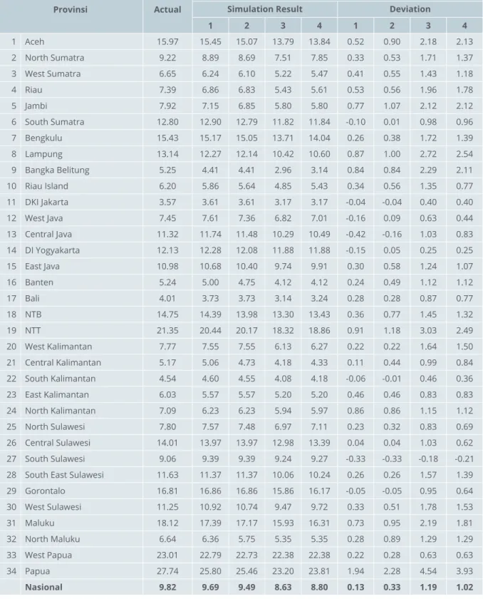
Table 6 Poverty Rate Simulation Result (March 2018)
Provinsi Actual
Scenario
Simulation Result Deviation
1 2 3 4 1 2 3 4
1 Aceh 15.97 15.45 15.07 13.79 13.84 0.52 0.90 2.18 2.13
2 North Sumatra 9.22 8.89 8.69 7.51 7.85 0.33 0.53 1.71 1.37
3 West Sumatra 6.65 6.24 6.10 5.22 5.47 0.41 0.55 1.43 1.18
4 Riau 7.39 6.86 6.83 5.43 5.61 0.53 0.56 1.96 1.78
5 Jambi 7.92 7.15 6.85 5.80 5.80 0.77 1.07 2.12 2.12
6 South Sumatra 12.80 12.90 12.79 11.82 11.84 -0.10 0.01 0.98 0.96
7 Bengkulu 15.43 15.17 15.05 13.71 14.04 0.26 0.38 1.72 1.39
8 Lampung 13.14 12.27 12.14 10.42 10.60 0.87 1.00 2.72 2.54
9 Bangka Belitung 5.25 4.41 4.41 2.96 3.14 0.84 0.84 2.29 2.11
10 Riau Island 6.20 5.86 5.64 4.85 5.43 0.34 0.56 1.35 0.77
11 DKI Jakarta 3.57 3.61 3.61 3.17 3.17 -0.04 -0.04 0.40 0.40
12 West Java 7.45 7.61 7.36 6.82 7.01 -0.16 0.09 0.63 0.44
13 Central Java 11.32 11.74 11.48 10.29 10.49 -0.42 -0.16 1.03 0.83
14 DI Yogyakarta 12.13 12.28 12.08 11.88 11.88 -0.15 0.05 0.25 0.25
15 East Java 10.98 10.68 10.40 9.74 9.91 0.30 0.58 1.24 1.07
16 Banten 5.24 5.00 4.75 4.12 4.12 0.24 0.49 1.12 1.12
17 Bali 4.01 3.73 3.73 3.14 3.24 0.28 0.28 0.87 0.77
18 NTB 14.75 14.39 13.98 13.30 13.43 0.36 0.77 1.45 1.32
19 NTT 21.35 20.44 20.17 18.32 18.86 0.91 1.18 3.03 2.49
20 West Kalimantan 7.77 7.55 7.55 6.13 6.27 0.22 0.22 1.64 1.50
21 Central Kalimantan 5.17 5.06 4.73 4.18 4.33 0.11 0.44 0.99 0.84
22 South Kalimantan 4.54 4.60 4.55 4.08 4.18 -0.06 -0.01 0.46 0.36
23 East Kalimantan 6.03 5.57 5.57 5.20 5.20 0.46 0.46 0.83 0.83
24 North Kalimantan 7.09 6.23 6.23 5.94 5.97 0.86 0.86 1.15 1.12
25 North Sulawesi 7.80 7.57 7.48 6.97 7.11 0.23 0.32 0.83 0.69
26 Central Sulawesi 14.01 13.97 13.97 12.98 13.39 0.04 0.04 1.03 0.62
27 South Sulawesi 9.06 9.39 9.39 9.24 9.27 -0.33 -0.33 -0.18 -0.21
28 South East Sulawesi 11.63 11.37 11.37 10.06 10.24 0.26 0.26 1.57 1.39
29 Gorontalo 16.81 16.86 16.86 15.86 16.17 -0.05 -0.05 0.95 0.64
30 West Sulawesi 11.25 10.92 10.74 9.47 9.72 0.33 0.51 1.78 1.53
31 Maluku 18.12 17.39 17.17 15.93 16.31 0.73 0.95 2.19 1.81
32 North Maluku 6.64 6.36 5.75 5.35 5.35 0.28 0.89 1.29 1.29
33 West Papua 23.01 22.79 22.73 22.38 22.38 0.22 0.28 0.63 0.63
34 Papua 27.74 25.80 25.46 23.20 23.81 1.94 2.28 4.54 3.93
Nasional 9.82 9.69 9.49 8.63 8.80 0.13 0.33 1.19 1.02
34
36
NATIONAL TEAM FOR THE ACCELERATION OF POVERTY REDUCTION Secretariat Office of the Vice President
Jl. Kebon Sirih Raya No.14, Central Jakarta, 10110 Telephone : (021) 391 2812
Fax : (021) 391 2511 Email : [email protected] Website : www.tnp2k.go.id