Patrice Maheo showed me by example how to get the most out of a free surface shear layer tunnel and he was a pleasure to work with. This study showed that the anisotropy known to exist in some other free-surface flows, such as surface-parallel submerged jets, is also present in the case of a mixing layer. In addition, the low-frequency spanwise oscillation is understood from the velocity power spectra and cospectra in the immediate vicinity of the mean streamwise vortices.
INTRODUCTION
I NTRODUCTION
Turbulence in the absence of mean shear has also been extensively studied near boundaries. Brown & Roshko (1974) identified the presence of coherent structures in the mixed layer and characterized their evolution. Banerjee (1994) and Pan & Banerjee (1995) investigated the behavior of turbulent updrafts impinging on a free surface and again noted that a quasi-two-dimensional region exists in the immediate vicinity of the surface. 1996) experimentally investigated a turbulent wake interacting with a free surface.
P RESENT O BJECTIVES
He used his downstream results to trace the origin of the surface layer back to the turbulent boundary layers along the splitter plate in both cases, with a Reynolds stress anisotropy driving the secondary flows. The flow in the bulk region – outside the influence of the free surface – was measured as a baseline. Second, there are the low-frequency oscillations associated with the fundamental instability of the mixing layer and possible oscillations in the surface currents that Maheo describes for this flow.
F LOW S ELECTION
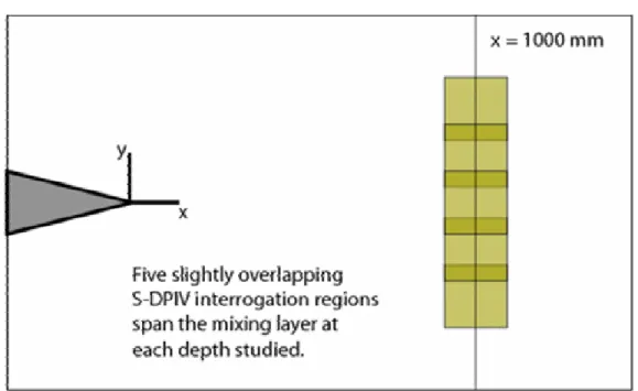
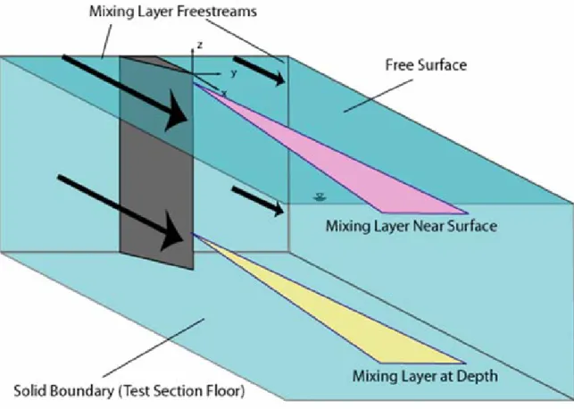
Thus, all six components of the Reynolds stress tensor, as well as the turbulence kinetic energy, can be obtained with one setup. A schematic of the flow and the regions to be investigated is shown in Figure 1.1. The specified downstream station to be studied, 1000 mm, was as far downstream from the tip of the manifold as the facility would support.
EXPERIMENTAL METHODS
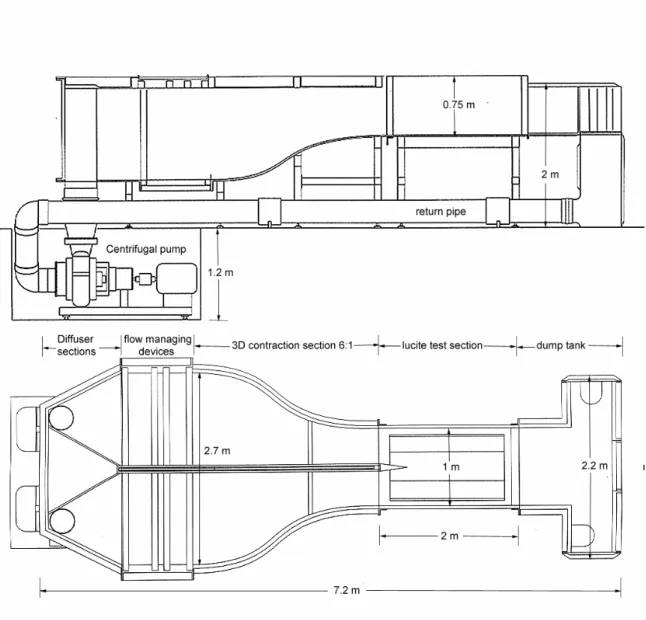
F ACILITY
The downstream end of the dump contains a plexiglass window that provides optical access directly behind the test piece. With the test section filled (as it was for these experiments), the maximum practical tunnel velocity was about 50 cm/s. This distribution board with a uniform cross-section from the floor of the test section to the top of the test section is shown in Figure 2.3.
P ARTICLE I MAGE D ATA A CQUISITION T ECHNIQUES
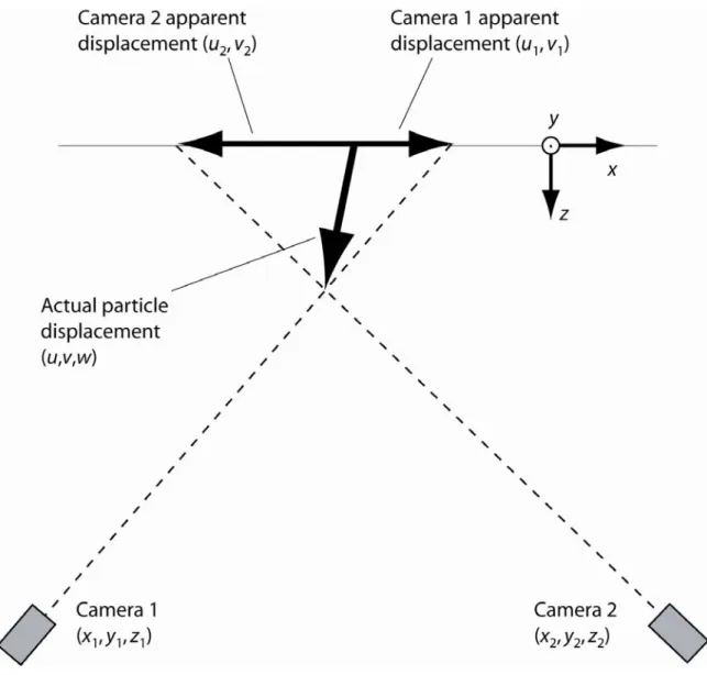
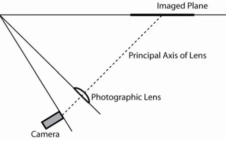
However, because of the added complexity, this is typically not done unless some peculiarity of the situation requires it. One obvious concern that cannot be ignored is the oblique image that each camera takes of the target area. There are two popular methods of dealing with problem (1) above, each of which involves repositioning the camera itself relative to the lens (Raffel et al., 1998).
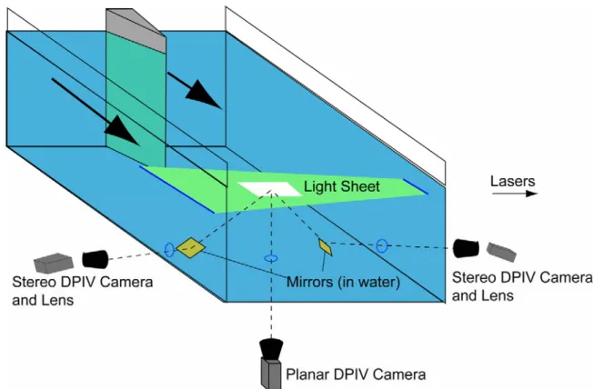
DPIV AND SDPIV AS A PPLIED
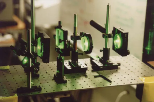
This equipment was placed directly on the side of the water tunnel and the laser light plate passed right through the Plexiglas side wall. The device visible on the far left of the platform, shown in Figure 2-8, consists of a pair of mirrors. At each measurement site (out of 25 in this series of experiments), several calibration images were recorded before and after the acquisition of the data images.
C OMPARISON OF 2-D AND S TEREO DPIV R ESULTS
REYNOLDS DECOMPOSITION
F LOW C HARACTERIZATION AT D EPTH
It is useful to note that the fluctuating part of the velocity components only appears in the last term in the RANS equations; all other terms are based on average amounts only. The arguments of the derivatives of this last term (ui'uj') are called the Reynolds stress. Reynolds voltages are elements of a tensor quantity in the RANS equations as given above; it is not uncommon to refer to the Reynolds stress tensor.
This is done using the finite difference routine that is part of the DPIV software package used. The transverse extent of the mixing layer at depth will be defined here by the eddy thickness, defined by . The evaluation of this quantity was quite simple based on the mean velocity data presented in the previous section: the calculation of the derivative of the mean velocity was done using a simple finite difference scheme.
For flows of this type, it has been shown to be appropriate to normalize the downstream distance by the moment thickness measured at the tip of the distribution plate (Maheo, 1998). It is also instructive to obtain estimates of what are often called the "intrinsic scales" of the flow—the scales at which viscous dissipation takes place. The velocity drain is easy to calculate from the available SDPIV data, and ν is the kinematic viscosity of the fluid.
This is approximately an order of magnitude smaller than the spatial resolution of the SDPIV data in this experiment.
F LOW P ROPERTY V ARIATIONS WITH D EPTH
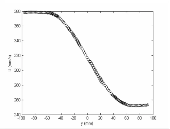
It is also clear that the width of the mixed layer varies strongly with depth. In the bulk flow, there is a pronounced area of mean flow in the direction of the free surface ( ), which more or less disappears in the intermediate depths shown. Near the free surface, this upwelling medium flow is seen to decrease significantly in magnitude.
It can be seen that the center of the vortex peak for all levels except that of the bulk stream is directed to the low-velocity side. When the width of the peak is reduced, the magnitude of the peak value is the same. It is seen that the magnitude of the peak value is significantly higher at z/δω = −0.25 than at any other depth.
This profile peak value outside the influence of the free surface is approx. 60 percent greater than u′w′ at the same depth. Many of the general trends observed in the individual component intensities can be seen, such as the pronounced narrowing of the profile and elevated peak value at z/δω = −0.25 and z/δω = −0.12. In the very near surface region, the total energy of the fluctuations is seen to take a profile similar to that in the bulk, but slightly wider and with a slightly lower peak value.
This value as a function of depth is plotted in Figure 3.23, where we see that the amount is almost independent of depth at all observed locations.
SPECTRAL ANALYSIS
T EMPORAL S PECTRA
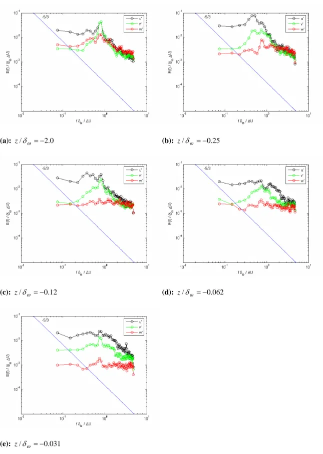
Of particular interest is the power spectral density (power spectra) of each of the three velocity components. The temporal frequency, f, was normalized by the bulk mixing layer parameters, as were the power spectra E (f). The dramatic increase in low-frequency streamwise motions (u) at this depth will be discussed in the next section.
A distinction that deserves attention is that here, when the free surface is approached from below, no appreciable increase in the higher frequencies of the streamwise velocity component is seen. Figure 4.3(a-e) again shows the same information, but this time as observed at y/δω = −0.75, in the direction of the high-speed free stream. The interest in this section is the characterization of the relatively low frequency oscillations which affect the mean and secondary flows known to exist in the free surface layer (Maheo, 1998).
This same reduction in apparent width of the mixing layer is also seen in the u and v plots. Similar behavior is observed in the spanwise fluctuations, but as the surface is approached there appears to be a. Figures 4.11(a-e) again present the same information, but this time as observed at y/δω = −0.75, in the direction of the high-speed free stream.
There are two distinct peaks in the u'v' cospectra at this depth, much like those seen at z/δω = -0.25.
C OMMENTS
On this basis, the transverse oscillation occurring near the free surface is assumed to have a magnitude that varies greatly with depth. We also note that the maximum apparent amplitude of this oscillation is at the depth that Maheo showed was approximately the depth at which two counter-rotating vortices appear in the mean flow. Given that such vortices also occur in the wakes of surface ships, and that the wakes of towed ships writhe (Shen, et al., 2002), a possible connection is clear.
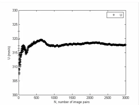
It has also been shown that a pair of counter-rotating eddies can exhibit instability and that the wavelengths at which the instability is most enhanced have been characterized (e.g., Crow, 1970). In the case studied here, the oscillation frequency as it passes from the measuring station at x = 1000 mm is approximately 0.8 s-1. Considering the convective velocity noted in chapter 3 of UC =316mm/s, we can conclude from this that the wave length in the direction of the oscillation flow is approximately 250mm.
The work of Widnall (1975) suggests that it would be the most unstable wavelength for such a vortex pair. This is much larger than the observed apparent wavelength, but it should also be noted that 650 mm is of the order of magnitude of the distance down at which the measurements are made. The mixing layer has been shown to grow more or less linearly with x, and Maheo's data show that the spacing between.
The closest analogue in the flow studied in this thesis to a radius is the only lateral length scale present, δω. This is similar to the wavelength of Shen et al., but the phenomena are somewhat. In the present work, on the other hand, the oscillation amplitude has a very pronounced peak value at a distance below the free surface and decreases as the surface is approached from below.
CONCLUSIONS
They also appear in a very similar way in the presented cospectra, especially in the spectrum of the streamwise and extensional velocity components. Strong parallels are seen with the wakes of towed model boats, particularly the close agreement in swing wavelength. In this section, representative examples of data convergence as the number of processed image pairs increases are presented.
Analysis of the data revealed the presence of what appears to be a standing wave very close to the surface on the high speed side of the tunnel. The most affected quantity was the mean vertical velocity W, which near the surface on the high-speed side of the tunnel exhibited strong variation in the streamwise direction. This particular location was among the worst affected and the cause is assumed to be a relatively low amplitude standing wave on the water surface.
Such deletions were limited to the high-speed side of the tunnel and at the two shallowest interrogation depths. The normalization of the co-spectrum results is done in the same vein as that for the power spectra. The value of ∆x varies slightly between measurement locations and is a function of processing details.
PSD normalization is exactly the same as that for temporal data as described above.