The Atmospheric Dynamics of Pulsar Companions
Adam S. Jermyn
Thesis Mentor: E. S. Phinney Option Representative: Lynne Hillenbrand
Division of Physics, Mathematics, and Astronomy California Institute of Technology
June 10, 2015
i Curiosity demands that we ask questions, that we try to put things together and try to understand this multitude of aspects as perhaps resulting from the action of a relatively small number of elemental things and forces acting in an infinite variety of combinations.
– Richard P. Feynman
Acknowledgements
Except where otherwise noted, and to the best of my knowledge, all work presented here is my own. Getting to this point, however, is something for which I am deeply indebted to those around me. Professor Sterl Phinney, my thesis mentor, taught me that intuition is more useful than precision, and patiently introduced me to the art of astronomy. Dr. Ravishankar Sundaraman, my collaborator and co-conspirator, showed me that numerical methods can be elegant as well as useful. Professor Jason Alicea, my adviser, introduced me to the subtle world of statistical physics, and gave me an appreciation for the many mysteries therein. Dr. Milo Lin, my friend and colleague, brought me into the fold of proteins and biophysics, and in so doing gave me my first taste of emergence. Dr. Frank Rice, my laboratory instructor, impressed upon me the importance of always being grounded in experiment and observation.
Professor Gil Refael, the leader of nights of free-wheeling physics and Thai food, gave me the firm belief that any problem in Nature may be solved with enough of both.
My friend Nicholas Schiefer gave me a little nudge towards astronomy in just the right way, and lent me an ear at all of the right times, and for that I will always be grateful. Of my professors and friends at Caltech, Tom Tombrello is the one I’ll never truly be able to thank. My adviser and advocate till the day he passed away, he believed in me even when I didn’t, and helped me find my way by gently pointing out the doors he had opened all around me. The other person I cannot thank properly is my grandfather Robert Katz, who passed away in May of 2014. He told me stories about the world through science and art and history, and in doing so piqued my curiosity. Finally, I would like to thank Mom and Dad. You set me on my way in this adventure.
Abstract
iv Pulsars emit radiation over an extremely wide frequency range, from radio through gamma1. Recently, systems in which this radiation significantly alters the atmospheres of low-mass pulsar companions have been discovered2. These systems, ranging from ones with highly anisotropic heating to those with transient X-ray emissions, represent an exciting opportunity to investigate pulsars through the changes they induce in their companions. In this work, we present both analytic and numerical work investigating these phenomena, with a particular focus on atmospheric heat transport, transient phenomena, and the possibility of deep heating via gamma rays. We find that certain classes of binary systems may explain decadal-timescale X-ray transient phenomena3, as well as the formation of so-called redback companion systems4. We also posit an explanation for the formation of high-eccentricity millisecond pulsars with white dwarf companions5. In addition, we examine the temperature anisotropy induced by the
1A. Smith David. “Gamma Ray Pulsars with the Fermi LAT”. in: 3rd Fermi Symposium. May 2011. url: http://fermi.gsfc.nasa.gov/science/mtgs/symposia/2011/program/session14/
Smith_FermiPSRs.pdf; H. et al Anderhub. “Search for Very High Energy Gamma-ray Emission from Pulsar-Pulsar Wind Nebula Systems with the MAGIC Telescope”. In: The Astrophysical Journal 710.1 (2010), p. 828. url: http://stacks.iop.org/0004- 637X/710/i=1/a=828; T.
Padmanabhan. Theoretical Astrophysics. Vol. 2. ISBN: 978-0521566315. Cambridge University Press, 2001. Chap. 6.
2Mallory S. E. Roberts. Surrounded by Spiders! New Black Widows and Redbacks in the Galactic Field. 2012. eprint: arXiv:1210.6903. url: http://arxiv.org/abs/1210.6903; M. T. Reynolds et al. “The light curve of the companion to PSR B1957+20”. In: Monthly Notices of the Royal Astronomical Society 379.3 (2007), pp. 1117–1122. doi: 10.1111/j.1365- 2966.2007.11991.x.
eprint: http://arxiv.org/abs/0705.2514. url: http://mnras.oxfordjournals.org/content/
379/3/1117.abstract.
3M. Linares. “X-Ray States of Redback Millisecond Pulsars”. In: The Astrophysical Journal 795, 72 (Nov. 2014), p. 72. doi: 10.1088/0004-637X/795/1/72. arXiv: 1406.2384 [astro-ph.HE].
4P. Podsiadlowski, S. Rappaport, and E. D. Pfahl. “Evolutionary Sequences for Low- and Intermediate-Mass X-Ray Binaries”. In: The Astrophysical Journal 565 (Feb. 2002), pp. 1107–
1133. doi: 10 . 1086 / 324686. eprint: astro - ph / 0107261; P. Podsiadlowski. “Irradiation- driven mass transfer low-mass X-ray binaries”. In: Nature 350 (Mar. 1991), pp. 136–138. doi: 10.1038/350136a0.
5B. Knispel et al. “Einstein@Home Discovery of a PALFA Millisecond Pulsar in an Eccentric Binary Orbit”. In: ArXiv e-prints(Apr. 2015). arXiv: 1504.03684 [astro-ph.HE].
v Pulsar in its companion, and demonstrate that this may be used to infer properties of both the companion and the Pulsar wind. Finally, we explore the possibility of spontaneously generated banded winds in rapidly rotating convecting objects.
Contents
Acknowledgements i
Abstract ii
Definition of Symbols ix
List of Figures xvii
Motivation 1
I Physics 5
1 Geometry and Optical Depth 6
2 One-Dimensional Model 14
2.1 Equations of Stellar Structure . . . 14
2.2 Simulations . . . 18
2.3 Luminosity and Radial Variation . . . 28
3 Higher Dimensional Models 36 3.1 Zero-Wind Analytic Model . . . 39
3.1.1 Iterative Method . . . 40
3.1.2 Eigenfunction Expansion . . . 42
3.2 Zero-Divergence Wind Model . . . 46
4 Review of Fluid Mechanics 49 4.1 Microscopic Viscosity . . . 49
4.2 Reynolds Number . . . 54
4.3 Rayleigh Number . . . 57 vi
CONTENTS vii
4.4 Richardson Number . . . 59
4.5 Rossby Number . . . 61
4.6 Mach Number . . . 62
5 Stability and Turbulence 65 5.1 Sheared Convection . . . 66
5.1.1 Shear-dominated flow . . . 69
5.1.2 Convection-dominated flow . . . 72
5.1.3 Mixed shear-convective flow . . . 73
5.2 Non-Convective Shear . . . 75
6 Global Wind Patterns 79 6.1 Turbulent Zonal Flow . . . 79
6.2 Alternative Patterns . . . 82
6.2.1 Large Rossby Number . . . 83
6.2.2 Small Rossby Number . . . 88
6.3 Deciding . . . 92
6.4 Convective Reynold’s Stress . . . 100
6.5 Summary of Results . . . 104
7 Higher Dimensional Models with Transport 110 7.1 Radiative Stars . . . 111
7.2 Convective Stars . . . 115
7.3 Crossover Behavior . . . 117
8 Time Dependence 125 8.1 Assumptions and Computational Methods . . . 125
8.2 Fully Radiative Stars . . . 129
8.3 Fully Convective Stars . . . 132
8.4 Mixed Stars . . . 138
II Applications in Astronomy 144
9 X-Ray Binaries 145 9.1 Accretion rate . . . 1459.2 Pre-Roche Expansion . . . 147
9.3 Post-Roche Accretion . . . 152
9.4 Critical Accretion Dynamics . . . 158
CONTENTS viii 9.5 Limit Cycles . . . 163
10 Accretion Induced Collapse 173
11 Spotted Black Widows 179
11.1 Setup . . . 180 11.2 Main Sequence Solutions . . . 183 11.3 Brown Dwarfs . . . 190
12 Banded Stars 198
Appendices 204
A Viscosity Code 204
B Acorn Stellar Integration Code 207
B.1 Opal and Ferguson Opacity Table Parser . . . 207 B.2 Stellar Integration Code . . . 211
C Gob Stellar Integration Code 239
D Anisotropy Code 266
E Reference Stellar Models 271
Bibliography 291
ix
Definition of Symbols
Symbol Name Definition/Value/[Units]
log Logarithm base 10 ln Logarithm base e
G Newton’s Constant 6.673×10⁻⁸ergcmg2
M Solar Mass 1.98855×1033g
R Solar Radius 6.955×10¹⁰m
L Solar Luminosity 3.83×1033erg/s
mp Proton Mass 1.6605×10⁻²⁴g
a Radiation Constant 7.57×10⁻¹⁵cmerg3K4
c Speed of Light 2.99792458×1010cm/s
kB Boltzmann Constant 1.38065×10⁻¹⁶erg/K
σ Stefan-Boltzmann Constant 5.6703×10⁻⁵erg/s/cm2/K4 Ry Rydberg - Hydrogen Ionization Energy 2.179872×10⁻¹¹erg
q Electron Charge Magnitude 4.80321×10⁻¹⁰√
erg·cm
M Stellar Mass [M]
Mp Pulsar Mass [M]
Σ Column Density [g/cm2]
Σh Heating Column Density [g/cm2]
κ Mass Attenuation Coefficient [cm2/g]
R Stellar Radius [R]
R0 Orbital Radius [cm]
Rb Roche Lobe Radius [cm]
P Orbital Period [s]
Pp Pulsar Rotation Period [s]
ω Pulsar frequency [rad/s]
z Depth [cm]
g Acceleration due to Gravity GMR2
P Pressure [erg/cm3]
ρ Density [g/cm3]
T Temperature [K]
u Specific Internal Energy [erg/cm3]
s Specific Entropy [erg/K/cm3]
Fb Flux due to Nuclear Processes [erg/cm2/s]
Lin Luminosity due to Nuclear Processes [erg/s]
Fr Radiative Flux 4acT3κρ3∂zT
Le External Luminosity [erg/s]
k Thermal Conductivity [erg/cm/s/K]
krad Radiative Thermal Conductivity 4acT3ρκ3 cv Specific Heat Capacity (Constant Volume) [kB/µ]
cp Specific Heat Capacity (Constant Pressure) γcv
γ Adiabatic Index ccp
v
µ Mean Free Particle Mass ρkTp
vs Speed of Sound qγpρ
hs Pressure Scale Height ddzlnp = ρgp
x
Symbol Name Definition/Value/[Units]
∇ Temperature Gradient ddlnlnTP
∇rad Radiative Temperature Gradient 4acGM T3κpFbr24
∇ad Adiabatic Temperature Gradient 1− γ1
l Convective Length-scale [cm]
ℵ Convective Scale Factor l/hs
Γ Convective Efficiency
∇conv Convective Gradient
vc Convective Speed [cm/s]
Fc Convective Flux Fnet−Fr
v0 Wind Speed
vφ Circumferential Wind Speed
∇c Circumferential Temperature Gradient ∂φlnT
∆z Region Thickness [cm]
τt Cooling Time Heat Content
Non-Transient Flux = cpTF(∆z)
b = γp(∆z)F
b
τw Wind Circulation Time 2πrv
w
ν Kinematic Viscosity [cm2/s]
N Brunt-Vaisala Frequency √
g∂zlnρ orqg∂zs/γ
Ri Richardson Number (dv/dz)N2 2
Ric Critical Richardson Number
Re Reynolds Number vd/ν with characteristic flow diameter d
Rec Critical Reynolds Number
β Thermal Expansion Coefficient [K−1]
α Thermal Diffusivity ck
p
Ra Rayleigh Number βglαν3∆T
Rac Critical Rayleigh Number ∼103
Pe Péclet Number vlα
r Spherical Radial Coordinate θ Spherical Polar Angle
φ Spherical Azimuthal/Cylindrical Polar Angle s Cylindrical Radial Angle
List of Figures
1.1 Depiction of a pulsar and its companion. Note that none of the depictions are to scale. The companion orbits with angular velocity equal to its rotational angular velocities due to tidal locking effects.
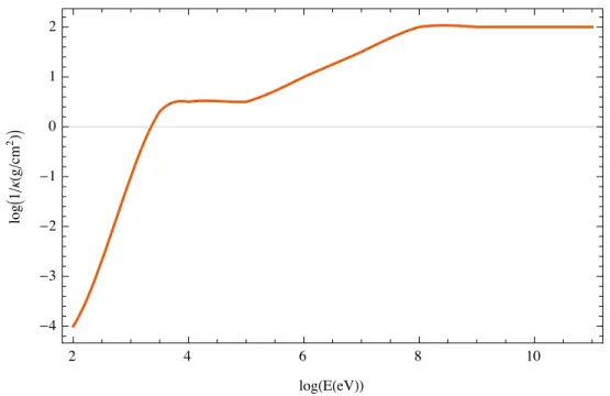
The pular and companion are separated by a distanceRo. Their masses are Mp and M respectively. The star has radius R. The heating zone is, for any kind of radiation, the region of unit optical depth given that the radiation is incident from one side and that the source is far enough away that it may be viewed as a planar wavefront. . . 8 1.2 logκ−1 is plotted versus logE. The former is measured in g/cm2 and
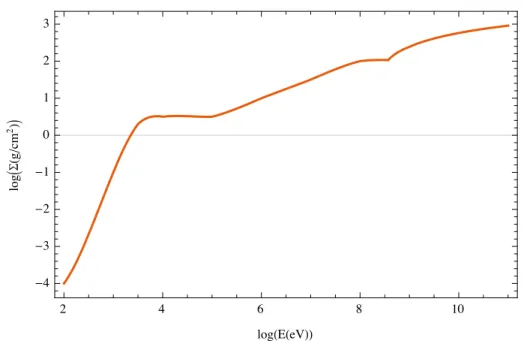
the latter in eV. Data was extracted manually from plots in the Particle Data Group book6, and so has some uncertainty associated with the conversion process. . . 10 1.3 log Σ is plotted versus logE. The former is measured in g/cm2 and
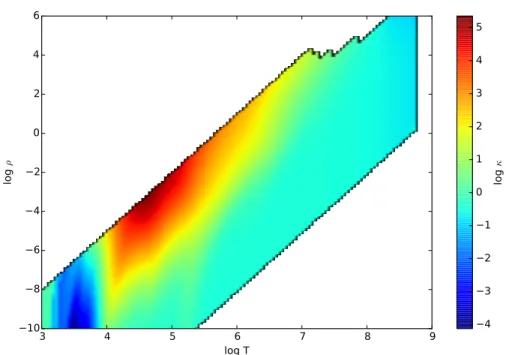
the latter in eV. . . 11 2.1 The vertical axis is logρ (with ρmeasured in g/cm3), the horizontal is
logT (with T measured in K), and the color represents logκ (withκ measured in cm2/g. White regions are those without data. . . 19
6´J. et al Beringer. “Particle Data Group”. In: Phys. Rev. D86 (2012), p. 010001.
xi
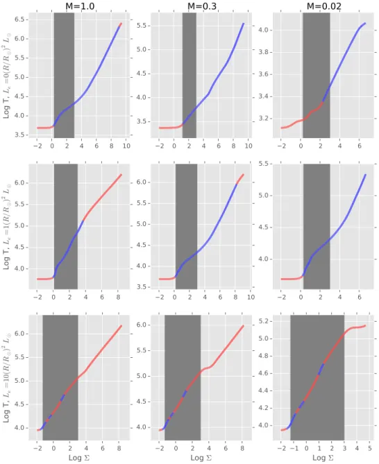
LIST OF FIGURES xii 2.2 Radial coordinate (in cm) versus log of Σ (in g/cm2) for nine different
scenarios. Σ here is computed as the mass above the point of interest divided by 4πR2. The columns are the three different stars under consideration. Moving left to right, they are M =M,Lin =L,R = R, M = 0.3M,Lin = 10−2L,R= 0.43R, and M = 0.02M,Lin = 10−4L,R = 0.14R. The rows represent different quantities of external luminosity. From top to bottom, these are Le= 0, Le=LR2
R
2, Le = 10LRR2
2. The vertical grey bar goes from the edge of the photosphere (where τ = 2/3) to the heating depth (Σ = 103g/cm2). Blue regions
are dominated by convective heat transport, red by radiative transport. 21 2.3 Log of T (in K) versus log of Σ (in g/cm2) for the same nine scenarios
defined in figure 2.2. Σ here is computed as the mass above the point of interest divided by 4πR2. The columns are the three different stars under consideration. The rows represent different quantities of external luminosity. The vertical grey bar goes from the edge of the photosphere (where τ = 2/3) to the heating depth (Σ = 103g/cm2). Blue regions
are dominated by convective heat transport, red by radiative transport. 23 2.4 Log of pressure scale height versus log of Σ (in g/cm2) for the same nine
scenarios defined in figure 2.2. The columns are the three different stars under consideration. The rows represent different quantities of external luminosity. The vertical grey bar goes from the edge of the photosphere (where τ = 2/3) to the heating depth (Σ = 103g/cm2). Blue regions
are dominated by convective heat transport, red by radiative transport. 24 2.5 Log of convective efficiency (Γ, see text) versus log of Σ (in g/cm2)
for the same nine scenarios defined in figure 2.2. The columns are the three different stars under consideration. The rows represent different quantities of external luminosity. The vertical grey bar goes from the edge of the photosphere (where τ = 2/3) to the heating depth (Σ = 103g/cm2). Blue regions are dominated by convective heat transport, and all other regions have been omitted due to Γ only being defined in convective zones. . . 26
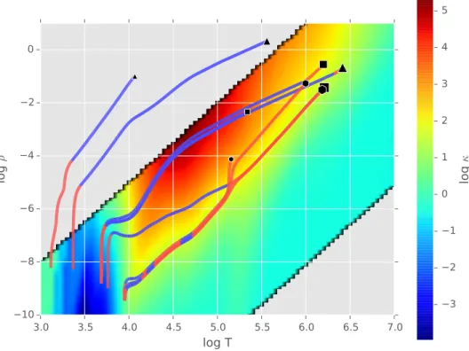
LIST OF FIGURES xiii 2.6 The vertical axis is logρ (with ρ measured in g/cm3), the horizontal
is logT (with T measured inK), and the color represents logκ (with κ measured in cm2/g. White regions are those without data. The nine stellar models defined in figure 2.2 are plotted as tracks on top of the opacity. The terminus marker indicates which track is which:
the three sizes of markers correspond in increasing order to the three stellar masses under consideration, and the three kinds of markers correspond in order of increasing number of sides to increasing external illumination. Blue regions are dominated by convective heat transport, red by radiative transport. . . 27 2.7 The log of f is plotted versus log(Le/Li,old) withβ = 4 + 2/3 in orange
and β = 0 in blue. These solutions were determined numerically in Mathematica. . . 33 4.1 The vertical axis is logρ (with ρmeasured in g/cm3), the horizontal is
logT (with T measured in K), and the color represents logν (with ν measured in cm2/s. White regions are those without data. . . 52 4.2 The vertical axis is logρ (with ρmeasured in g/cm3), the horizontal is
logT (withT measured inK), and the color represents the log of the anisotropy factor A. White regions are those without data. . . 55 4.3 The vertical axis is logρ (with ρmeasured in g/cm3), the horizontal is
logT (withT measured inK), and the color represents the log of the anisotropy factor A. White regions are those without data. . . 56 8.1 ∆T /T0 (top) and L/L (bottom) versus log Σ (in g/cm2) for a star of
mass M, radius R, and luminosity 100L. The external heat was put in at Σ = 103g/cm2 and linearly increased from zero to 100L
over the course of 108s, which is where the simulation ends. Color represents time, with the simulation beginning at violet and ending with red. . . 130 8.2 ∆T /T0 (top) and L/L (bottom) versus log Σ (in g/cm2) for a star of
massM, radiusR, and luminosity 100L. The external heat was put in at Σ = 103g/cm2 and linearly increased from zero to 100Lover the course of 108s, after which the simulation continued for another 108s to allow for equilibration. Color represents time, with the simulation beginning at violet and ending with red. . . 131
LIST OF FIGURES xiv 8.3 ∆T /T0 (top) and L/L (bottom) versus log Σ (in g/cm2) for a star of
mass M, radius R, and luminosity 100L. The external heat was put in at Σ = 103g/cm2 and linearly decreased from 100L to zero over the course of 108s. Color represents time, with the simulation beginning at violet and ending with red. . . 133 8.4 ∆T /T0 (top) and L/L (bottom) versus log Σ (in g/cm2) for a star of
mass 0.3M, radius 2.65R, and luminosity 0.1L. The external heat was put in at Σ = 103g/cm2 and linearly decreased from 0.1L to zero over the course of 108s. Color represents time, with the simulation beginning at violet and ending with red. . . 134 8.5 ∆T /T0 (top) and L/L (bottom) versus log Σ (in g/cm2) for a star
of mass 0.3M, radius 2.65R, and luminosity 0.1L. The external heat was put in at Σ = 103g/cm2 and linearly decreased from 0.1L
to zero over the course of 108s. The simulation was then run for an additional 108s with no external heating. Color represents time, with the simulation beginning at violet and ending with red. . . 135 8.6 ∆T /T0 (top) and L/L (bottom) versus log Σ (in g/cm2) for a star
of mass 0.3M, radius 2.65R, and luminosity 0.1L. The external heat was put in at Σ = 103g/cm2 and linearly decreased from L
to zero over the course of 108s. The simulation was then run for an additional 108s with no external heating. Color represents time, with the simulation beginning at violet and ending with red. . . 136 8.7 ∆T /T0 (top) and L/L (bottom) versus log Σ (in g/cm2) for a star of
mass M, radius R, and luminosity L. The external heat was put in at Σ = 103g/cm2 and linearly decreased fromL to zero over the course of 108s. Color represents time, with the simulation beginning at violet and ending with red. . . 140 8.8 ∆T /T0 (top) and L/L (bottom) versus log Σ (in g/cm2) for a star
of mass 0.3M, radius 2.65R, and luminosity 0.1L. The external heat was put in at Σ = 103g/cm2 and linearly decreased from 10L to zero over the course of 108s. The simulation was then run for an additional 108s with no external heating. Color represents time, with the simulation beginning at violet and ending with red. . . 141
LIST OF FIGURES xv 8.9 ∆T /T0 (top) and L/L (bottom) versus log Σ (in g/cm2) for a star of
mass M, radius R, and luminosity L. The external heat was put in at Σ = 103g/cm2 and linearly decreased fromL to zero over the course of 108s. It was then run for another 108s at that value. Color represents time, with the simulation beginning at violet and ending with red. . . 142 8.10 ∆T /T0 (top) and L/L (bottom) versus log Σ (in g/cm2) for a star of
mass M, radius R, and luminosity L. The external heat was put in at Σ = 103g/cm2 and immediately decreased from L to zero over the course of 108s before being run for another 109s. Color represents time, with the simulation beginning at violet and ending with red. . . 143 9.1 The vertical axis is logP in seconds, the horizontal axis is the com-
panion mass M in solar masses, and the color represents the log of the expansion timescale hs/R˙ in seconds. The four different plots correspond to four different pulsar luminosities. . . 153 9.2 The vertical axis is logP in seconds, the horizontal axis is the com-
panion mass M in solar masses, and the color represents the log of τdisk/τexp. The four plots correspond to different pulsar luminosities. . 157 9.3 The vertical axis is logP in seconds, the horizontal axis is the com-
panion mass M in solar masses, and the color represents the log of the ratio of the quick contraction length to the scale height. The four plots correspond to different pulsar luminosities. . . 161 9.4 The vertical axis is logP in seconds, the horizontal axis is the com-
panion mass M in solar masses, and the color represents the log of the contraction timescale. The four plots correspond to different pulsar luminosities. . . 162 9.5 The vertical axis is logP in seconds, the horizontal axis is the com-
panion mass M in solar masses, and the color represents the log of the ratio of the critical disk viscous timescale to the contraction timescale.
The four plots correspond to different pulsar luminosities. . . 164 9.6 The vertical axis is logP in seconds, the horizontal axis is the com-
panion mass M in solar masses, and the color represents the type of limit cycle. Blue is type 1, Green is type 2, Maroon is type 3. The four plots correspond to different pulsar luminosities. . . 169
LIST OF FIGURES xvi 10.1 The vertical axis is M/M, the horizontal axis is Mc/M, with both
axes log-scaled. The color represents the ratio Rmax/30R, the denom- inator being the approximate Roche radius for the period and mass range of interest, and the numerator being the post-expansion radius of the red giant of interest. . . 177 11.1 The vertical axis is P in seconds, the horizontal axis is the companion
mass in solar masses, with both axes log-scaled. The color represents the log of the day/night flux ratio logFday/Fnight. The four different plots correspond to four different pulsar luminosities. The black line corresponds to the Roche cutoff. . . 186 11.2 The vertical axis is P in seconds, the horizontal axis is the companion
mass in solar masses, with both axes log-scaled. The color represents the log of the day/night flux ratio log ∆F/F. The four different plots correspond to four different pulsar luminosities. The black line corresponds to the Roche cutoff. The white regions above the Roche cutoff have ∆F = 0 due to heat bottling. . . 187 11.3 The vertical axis is P in seconds, the horizontal axis is the companion
mass in solar masses, with both axes log-scaled. The color represents the log of the day/night flux ratio logFday/(Fi+Fe). The four different plots correspond to four different pulsar luminosities. The black line corresponds to the Roche cutoff. . . 188 11.4 The vertical axis is P in seconds, the horizontal axis is the companion
mass in solar masses, with both axes log-scaled. The color represents the log of the day/night flux ratio logW/(Fi+Fe). The four different plots correspond to four different pulsar luminosities. The black line corresponds to the Roche cutoff. Note that the white region above the Roche cutoff corresponds to the case W = 0 . . . 189 11.5 The vertical axis is P in seconds, the horizontal axis is the companion
mass in solar masses, with both axes log-scaled. The color represents the log of the day/night flux ratio logFnight/Fi. The four different plots correspond to four different pulsar luminosities. The black line corresponds to the Roche cutoff. . . 191 11.6 Top: ∆F/Fe is shown as a function of logχ. Bottom: logFday/Fnight
is shown as a function of logχ. . . 194
List of Tables
6.1 Computed parameterization of circumferential heat transport by winds.
The first column specifies what case is under consideration. All pos- sible cases are enumerated here. The remaining columns specify y, a prefactor on the transport as well as q, a, b, the exponents on ∆T /T, l/2πR, and Ro respectively. Note that factors of γ and ℵ have been neglected in assembling this table. . . 105 6.2 Critical thermal anisotropy values are listed for each case of interest.
Note that factors of γ and ℵ have been neglected in assembling this table. . . 107
xvii
Motivation
If you haven’t found something strange during the day, it hasn’t been much of a day.
– John Archibald Wheeler Pulsars, highly magnetic compact stellar remnants, exhibit some of the most un- usual behaviors in the universe by virtue of existing at length and energy scales where general relativity and quantum field theory are both relevant. Pulsar gravitational fields are typically so strong that in binary pairs they emit significant gravitational radiation. The magnetic field near a pulsar’s surface is strong enough that the index of refraction of the vacuum deviates significantly from unity, and particle pair creation helps create an ionized wind which travels relativistically away from the pulsar7.
Most of what is known of pulsars comes from radio timing data8. Pulsars may be thought of as spherical magnetic dipoles approximately 10km in radius with surface magnetic fields between 108Gauss and 1015Gauss, spinning with periods between millisecond and second timescales9. As a result of the large electric fields created by the rotating magnetic dipole moment, particles are created and carry energy, both kinetic and in the form of a Poynting flux, away from the pulsar. As these particles move they also radiate gamma-rays. Observationally, this means that pulsars appear in a wide band of radio frequencies as a periodic short pulse, while also being active through very high energies. The timing of these pulses has informed much of what is currently known about pulsars.
7Padmanabhan, op. cit.
8Dipankar Bhattacharya. “The Evolution of the Magnetic Fields of Neutron Stars”. In: J.
Astrophys. Astr. 16 (Mar. 1994), pp. 217–232. url: http://www.ias.ac.in/jarch/jaa/16/217- 232.pdf.
9Idem, “The Evolution of the Magnetic Fields of Neutron Stars”; José A. Pons et al. “Evidence for Heating of Neutron Stars by Magnetic-Field Decay”. In: Phys. Rev. Lett. 98 (7 Feb. 2007), p. 071101. doi: 10.1103/PhysRevLett.98.071101. eprint: http://arxiv.org/pdf/astro- ph/0607583.pdf?origin=publication_detail. url: http://link.aps.org/doi/10.1103/
PhysRevLett.98.071101.
1
2 More specifically, pulsars have masses and radii in a very small range constrained by models of the degenerate nuclear equation of state10. From dispersion delay data at different frequencies it is possible to determine the electron column density in the interstellar medium between Earth and the pulsar, which can give a distance estimate11. Measurement of the pulse period gives the angular frequencyω. Combined with the mass and radius this gives the rotational energy of the pulsar:
E = 1
2Iω2 = 1
5M R2ω2 (1)
Measurement of the rate at which the pulse period changes gives ˙ω, which then gives the rate at which the pulsar rotational energy changes:
E˙ = 2
5M R2ωω˙ (2)
Equating this with the energy loss rate of a magnetic dipole then gives the surface dipole magnetic field. Measurement of ˙ω can also give insight into the mechanisms transferring angular momentum to or from the pulsar by giving an estimate of the braking index12.
While these techniques give significant insight into the properties of the pulsar, they give very little information regarding the surrounding environment. In particular, the properties of the pulsar wind are currently not very well known. While it is known that some fraction of the outgoing electromagnetic flux must be converted into a particle flux at the light cylinder of radius
Rl= c
ω, (3)
little is known of the nature of this conversion and the effect it has on the radiation portion of the energy flux. Recently, a number of binary systems composed of a pulsar and star orbiting it have been discovered in which the pulsar wind causes observable changes in the companion star13. If the companion star has a mass less
10Padmanabhan, op. cit.; J. M. Lattimer and M. Prakash. “Neutron Star Structure and the Equation of State”. In: The Astrophysical Journal 550.1 (2001), p. 426. eprint: http://arxiv.
org/abs/astro-ph/0002232. url: http://stacks.iop.org/0004-637X/550/i=1/a=426.
11Andrea N Lommen and Paul Demorest. “Pulsar timing techniques”. In: Classical and Quantum Gravity 30.22 (2013), p. 224001. eprint: http : / / arxiv . org / abs / 1309 . 1767. url: http : //stacks.iop.org/0264-9381/30/i=22/a=224001.
12Padmanabhan, op. cit.
13R. P. Breton et al. “Discovery of the Optical Counterparts to Four Energetic Fermi Millisecond Pulsars”. In: The Astrophysical Journal 769 (2013), p. 108. url: http://arxiv.org/abs/1302.
1790.
3 than the 0.08M minimum required to sustain fusion, the system is known as a Black Widow14, and if the pulsar wind heats the companion and causes it to swell to fill its Roche lobe, the system is known as a Redback15.
In the vast majority of Black Widows, even heating is seen on the pulsar-facing side16. There is one, however, known as PSR J1544-4937, in which the heating appears to be highly concentrated towards a small set of points on the companion.
This indicates effects involving the interaction between the wind and the companion magnetosphere.
In the case of Redbacks, it is possible that Roche lobe-filling companions can begin an accretion process onto the pulsar as a result of heating from the wind. If this occurs, the system can become an X-ray binary. There are several known cases of X-ray binaries which turn on and off on timescales of∼10yrs17. This may be due to the accretion disk burying the magnetic field of the pulsar, allowing the companion to cool and thereby halting the accretion process18. Under this model, when the accretion rate drops sufficiently the process begins again.
Both kinds of systems offer an opportunity to learn more about the pulsar wind, in particular as the effects of the wind on the companion are strongly influenced by its composition. For typical low-frequency radiation (anything ranging up to X-rays in energy), the region which the wind heats is in the upper atmosphere of the star, near the photosphere. The result is that the radiation is just re-radiated without significantly altering the structure of the atmosphere. The net effect is a rise in
14Roberts, op. cit.; D. J. Stevenson. “The search for brown dwarfs”. In: Annual Review of Astronomy and Astrophysics 29 (1991), pp. 163–193. doi: 10 . 1146 / annurev . aa . 29 . 090191 . 001115.
15Hai-Liang Chen et al. “Formation of Black Widows and Redbacks—Two Distinct Populations of Eclipsing Binary Millisecond Pulsars”. In: The Astrophysical Journal 775.1 (2013), p. 27. eprint:
http://arxiv.org/abs/1308.4107. url: http://stacks.iop.org/0004-637X/775/i=1/a=27.
16Reynolds et al., op. cit.; Roger W. Romani et al. “PSR J1311–3430: A Heavyweight Neutron Star with a Flyweight Helium Companion”. In: The Astrophysical Journal Letters 760.2 (2012), p. L36.
eprint: http://arxiv.org/abs/1210.6884. url: http://stacks.iop.org/2041-8205/760/i=
2/a=L36; M. H. van Kerkwijk, R. P. Breton, and S. R. Kulkarni. “Evidence for a Massive Neutron Star from a Radial-velocity Study of the Companion to the Black-widow Pulsar PSR B1957+20”.
In: The Astrophysical Journal 728.2 (2011), p. 95. eprint: http://arxiv.org/abs/1009.5427.
url: http://stacks.iop.org/0004-637X/728/i=2/a=95.
17Icdem, B. and Baykal, A. “Viscous timescale in high mass X-ray binaries”. In: Astronomy and Astrophysics 529 (2011), A7. doi: 10.1051/0004-6361/201015810. eprint: http://arxiv.org/
abs/1102.4203. url: http://dx.doi.org/10.1051/0004-6361/201015810.
18J. Hessels. “M28I and J1023+0038: The Missing Links Go Missing, but Provide a New Link”. In:
NS Workshop. Dec. 2013. url: http://www.astro.uni-bonn.de/NS2013-2/Hessel_M28i.pdf.
4 temperature on the near-side according to the Stefan-Boltzmann law:
4πR2σTnew4 = 4πR2σTold4 +Le. (4) The far-side does not heat at all, as there is no time to move the absorbed heat around the star before reemission occurs.
When the radiation is higher in energy, or is made of massive particles, the situation is somewhat different. High energy radiation can penetrate quite deep into the star, as will be discussed later. Massive particles can likewise make it quite far, particularly if they are uncharged. Charged massive particles are, however, limited by the ionization zone in how far they may travel. Regardless of the specific form of the external heating, when it occurs at depth the picture is very different. In particular, the heat has some time to be redistributed within the star rather than immediately escaping to the near-side. The formal statement of this effect is that the time it takes for the heat to be nontrivially redistributed is now comparable to or shorter than the radiative relaxation time. Profound structural changes in the stellar atmosphere may occur, including the excitation of gravity waves, strong zonal winds, tropical hurricanes, and the inducement of swelling in the deeper regions of the atmosphere.
This last symptom of external heating may be responsible for the observed Roche-lobe filling in certain Redback systems, with the eponymous thermal difference on the surface between the two sides of the star being due to the non-penetrative flux of the Pulsar wind.
As these phenomena couple heat transport, fluid mechanics, orbital mechanics, and various pieces of thermodynamic microphysics, we will discuss the physics first, and then the astronomy. Along the way, we will use examples from astronomy to illustrate relations, gain intuition, and build models, but only at the end will the astrophysical phenomena of interest be discussed in full.
Part I Physics
5
1
Geometry and Optical Depth
6
1. GEOMETRY AND OPTICAL DEPTH 7
, .
There is geometry in the humming of the strings, there is music in the spacing of the spheres.
– Pythagoras The geometry of the situations of interest is outlined in Fig. 1.1. The companion star and pulsar orbit their center of mass with angular velocity Ω. The companion is tidally locked, and hence Ω is also its rotation rate. The pulsar, on the other hand, has rotation rateω Ω. The two objects are separated by distance Ro, and have masses Mp andM for the pulsar and companion respectively. The star has radius R.
Note that the relative distances depicted are not shown to scale. The heating zone is, for any kind of radiation, the region surrounding the surface of unit optical depth. In the cases of interest the source is positioned on one side of the companion and is far enough away that it may be viewed as roughly a planar wavefront.
To determine where the heating zone lies, we must examine the optical depth associated with various kinds of radiation incident on the surface of the star. Below 10keV, the chief scattering processes are resonant absorption and Rayleigh scatter- ing1. Above this scale, Compton scattering becomes the dominant process,until approximately 1MeV∼2me, at which point the dominant process is pair production.
This state of affairs continues to arbitrarily high energies once the electron-positron pair production threshold is crossed. The use of the pair production decay channel, however, means that there will be more particles present after the initial scattering, and these may continue moving through the star for some distance before further scattering thermalizes them. If the resulting particles have energies above some critical level, the dominant process once all channels and possibilities are accounted for will continue to be pair production.
The net result of all of this is that for incident radiation below a critical energy, a single scattering event suffices and the cross-section directly gives the depth at which the radiation deposits heat. This gives
Σ = 1
κ, (1.1)
where κis the mass attenuation coefficient corresponding to the material and particle kind. Above the critical energy, the resulting particles from the first scattering continue to produce further particles until their descendents drop below the critical energy and produce heat. At each stage in the shower, additional particles are produced with energies approximately two times lower than what they started with, so if Eγ
1J. et al Beringer. “Particle Data Group”. In: Phys. Rev. D 86 (2012), p. 010001.
1. GEOMETRY AND OPTICAL DEPTH 8
R
Ro
Mp M
Ω
Heating Zone
Pulsar Companion Star
ω Ω
Figure 1.1: Depiction of a pulsar and its companion. Note that none of the depictions are to scale. The companion orbits with angular velocity equal to its rotational angular velocities due to tidal locking effects. The pular and companion are separated by a distanceRo. Their masses areMp and M respectively. The star has radius R.
The heating zone is, for any kind of radiation, the region of unit optical depth given that the radiation is incident from one side and that the source is far enough away that it may be viewed as a planar wavefront.
1. GEOMETRY AND OPTICAL DEPTH 9 is the energy of the photon and Ecrit is the critical energy, a total of approximately log2(Eγ/Ecrit) are created. If the scattering cross-section at each stage is roughly constant, as is expected in the case of energies above GeV scales2, then this means that the column density at which heat is produced should be
Σ = 1 κ
1 + log2 Eγ Ecrit
, The critical energy is given approximately3 in gases by
Ecrit= 710MeV Z + 0.92,
where Z is the number of protons in a nucleus. For hydrogen this simplifies to Ecrit= 370MeV.
Plots ofκ−1 and the corresponding Σ are shown in Fig. 1.2 and Fig. 1.3 respectively.
For hydrogen, the value of κ−1 is approximately 100g/cm2 for all energies beyond Ecrit which have been measured5, going up through 100GeV. Thus
Σ = 100 g cm2
1 + log2 Eγ 370MeV
.
Typical pulsar photon energies in the upper end of the spectrum are of order hundreds of GeV6. Substituting this in gives roughly
Σh = 103 g
cm2. (1.2)
This is the column density at which a stellar companion transforms the pulsar’s gamma rays into heat, and we will use this value in calculations involving the heating depth. To most appropriately model the physical process of particle showers and absorption, we will treat the incident luminosity as following
Le(Σ) =Lee−Σ/Σh, (1.3)
2Ibid.
3Ibid.
5Ibid.
6A. Smith David. “Gamma Ray Pulsars with the Fermi LAT”. in: 3rd Fermi Symposium. May 2011. url: http://fermi.gsfc.nasa.gov/science/mtgs/symposia/2011/program/session14/
Smith_FermiPSRs.pdf; H. et al Anderhub. “Search for Very High Energy Gamma-ray Emission from Pulsar-Pulsar Wind Nebula Systems with the MAGIC Telescope”. In: The Astrophysical Journal710.1 (2010), p. 828. url: http://stacks.iop.org/0004-637X/710/i=1/a=828.
1. GEOMETRY AND OPTICAL DEPTH 10
Figure 1.2: logκ−1 is plotted versus logE. The former is measured in g/cm2 and the latter in eV. Data was extracted manually from plots in the Particle Data Group book4, and so has some uncertainty associated with the conversion process.
1. GEOMETRY AND OPTICAL DEPTH 11
Figure 1.3: log Σ is plotted versus logE. The former is measured in g/cm2 and the latter in eV.
where Le measures only the high-energy photons. Low energy photons are ignored, as they are absorbed and reemitted soon thereafter in the photosphere.
Armed with this information regarding the structure of the heating zone, we can in principle take a three-dimensional model of a star and compute the spatial dependence of the heating. Again, in principle, this may be used to compute the resulting effects on the star. For the purposes of gaining physical intuition, however, this is not the most effective way to proceed, for there are many simplifications which may save substantially on computational effort and may make clearer the relevant physics.
The most basic model for the companion star which captures some of the physics of interest is to treat it as one-dimensional, and ignore the azimuthal symmetry breaking which results from the tidal locking. In this case, the star is parametrized by a series of functions of the radial coordinate, such as temperature, pressure, and so on.
Though this model neglects a significant physical asymmetry, it is advantageous in its mathematical and computational simplicity, and so will be our starting point. Within the context of this model, we will treat all physical quantities as their averages over the angular coordinates, such that the externally incident flux will sum up to the same total luminosity. As a result, this model is often referred to as the plane-parallel or isotropic atmosphere, for in it there is only one coordinate (depth) which matters.
1. GEOMETRY AND OPTICAL DEPTH 12 After this model, the next modification will be to examine higher-dimensional models. We will examine both two-dimensional models which add just the azimuthal coordinate φ and fully three dimensional models. In the former, we will treat all quantities as their average over the spherical polar angle θ, while the latter holds the full dimensionality of the system.
Beyond spatial dimensions, there is also the question of time. Initially we will consider all solutions in the steady-state. After this, we will shift to considering the time-dependence of these models, and exa mine both the stability of the steady-state solutions and the means by which they are reached.
1. GEOMETRY AND OPTICAL DEPTH 13
References
Anderhub, H. et al. “Search for Very High Energy Gamma-ray Emission from Pulsar- Pulsar Wind Nebula Systems with the MAGIC Telescope”. In: The Astrophysical Journal 710.1 (2010), p. 828. url: http://stacks.iop.org/0004-637X/710/i=
1/a=828(cit. on p. 9).
Beringer, J. et al. “Particle Data Group”. In: Phys. Rev. D 86 (2012), p. 010001 (cit. on pp. 7, 9).
Smith David, A. “Gamma Ray Pulsars with the Fermi LAT”. In: 3rd Fermi Symposium.
May 2011.url:http://fermi.gsfc.nasa.gov/science/mtgs/symposia/2011/
program/session14/Smith_FermiPSRs.pdf (cit. on p. 9).
2
One-Dimensional Model
There is a computer disease that anybody who works with computers knows about. It’s a very serious disease and it interferes completely with the work. The trouble with computers is that you "play" with them!
– Richard P. Feynman1
2.1 Equations of Stellar Structure
In the isotropic steady-state model, we treat all quantities in the companion as functions ofr, the distance from its center. No other independent variable enters in this model, astis forbidden by the steady-state assumption andθandφare forbidden by the isotropy assumption. Thus we write temperature asT(r), pressure as P(r), and so on.
To a very good approximation, we may neglect the variation in the composition of the star with position. That is, we treat all compositional variables as global constants, such thatX(r) = X0, the hydrogen mass fraction in the star, and likewise for all other such quantities. In making this approximation we mainly lose accuracy in calculating the properties of convection zones, though there our accuracy is primarily limited by the uncertainty in the choice of mixing length, and so this loss is acceptable.
The remaining spatial variables are then only thermodynamic ones. Of these, one might pick as "fundamental" ones the pressure, temperature, density, and mean
1Richard P. Feynman. Los Alamos From Below. https : / / www . youtube . com / watch ? v = 0ogSC6JKkrY. Feb. 6, 1975. url: http : / / calteches . library . caltech . edu / 34 / 3 / FeynmanLosAlamos.htm.
14
2. ONE-DIMENSIONAL MODEL 15 molecular weight2. All other quantities of interest may be derived from these. We may, however, eliminate µ, for it is a direct function of T. This follows from the fact that we have held compositional variables fixed, such that µvaries only through ionization.3. This variation occurs mainly when kBT is comparable to 13.6eV, and is generally taken to happen between 103.8K and 104.1K. The value of 13.6eV, of course, is the ionization energy of hydrogen.
Using the equation of state, we may eliminate yet another function, to reduce the total count of "fundamental" thermodynamic variables at each point to two. The equation of state is most generally written as
P =f(ρ, T), (2.1)
though it is usually well approximated by the form µP =ρkBT +1
3aT4, (2.2)
where the second term is included to accommodate radiation pressure. At low temperatures the second term may be dropped, yielding the familiar ideal gas law.
Regardless of the specific form, we will use the equation of state to eliminate the density from consideration, and hence write
ρ=g(P, T). (2.3)
Our ability to write it in this form comes from P being monotonic in ρ andT. We chooseρ rather than T or P because we generally wish to compute heat transport properties in terms of temperature, and in hydrostatic equilibrium the pressure is computable by a straightforward integral. As a result, we are left with two basic functions, P(r) and T(r), which fully characterize the star to within our various approximations.
It will often be more convenient to replace r withm, the mass above a particular radius, as the independent variable. As m is monotonically decreasing with r this is a perfectly well-defined transformation. We thus writeP =P(m), T =T(m). In this language, the condition of hydrostatic equilibrium may be cast into a convenient form, as
dP
dr =−ρg → dP
dm = g
4πr2. (2.4)
Now over the depth ranges of interest, as will be verified later,r varies only slightly relative to R. As a result, we may neglect its variation in computing quantities
2Other valid choices include specific energy, specific entropy, sound speed, etc.
3At high pressures it may also depend on pressure, and indeed we will account for this
2. ONE-DIMENSIONAL MODEL 16 in which r appears as a multiplicative factor. This is known as the thin-envelope assumption, and has several useful implications. For instance, we may approximate the gravity of the star as being fixed at
g ≡ GM
R2 . (2.5)
As a result, we may write the condition of hydrostatic equilibrium as dP
dm = GM
4πR4. (2.6)
Using the boundary conditionP(r=∞) = 0, m(r =∞) = 0 we find P(m) = GM m
4πR4 . (2.7)
Note that we may also use the variable
Σ≡ m
4πR2 (2.8)
as the independent variable. Given that this is the form in which we know the heating depth, we will often switch to using this rather thanm.
Given T(m), in addition to what we have found so far, we will know the structure of the star to within the bounds of our approximations. As a result, we know that T(m) must depend in some fashion on the luminosity of the star and on the external illumination we hope to investigate, for these quantities appear nowhere else and they seem quite important. To that end, consider the outer boundary condition on the star. There are a variety of models for this4, but most treat the low-m regime by some gas-radiation dilution model and use this to find the optical depth along the radial direction. From there, it is typically asserted that
L= 4πR2σT4 (2.9)
at the place where the optical depth τ = 2/3. This is just an application of the Stephan-Boltzmann radiation law to a gray-body atmosphere, with an effective treatment for the differing rates at which different frequencies of radiation escape at low optical depth. We will not go into the specific details of the model we used, and merely state that they are those described in Ref.5.
4B. Paczyński. “Envelopes of Red Supergiants”. In: Acta Astronomica 19 (1969), p. 1.
5Ibid.
2. ONE-DIMENSIONAL MODEL 17 From this upper boundary condition on T, we may integrate towards higher m using the equation
dT
dm = dlnT dlnP
!T P
dP
dm =∇T P
dP
dm, (2.10)
where the second equality defines the symbol∇and where the derivative with respect to lnP is taken along the radial direction. This last point is not relevant in an isotropic star, where ∇T and ∇p are aligned, but will become important when we move to higher dimensional models.
Of course, there is no physical content in Eq. (2.10): it is simply a true statement regarding differentiable functions. The reason we bother to cast the problem in this form is that∇ may often be expressed simply. In regions of the star where heat is transported radiatively,
∇=∇rad = 3κP L
16πacGM T4, (2.11)
where κ is the Rosseland mean opacity of the stellar material, and is generally a function ofP andT. On the other hand, when the region of interest is unstable against convection, the thermal gradient∇ is somewhat more complicated. If convection is efficient, then the convective gradient matches the adiabatic gradient, such that
∇=∇ad = dlnT dlnP
s
. (2.12)
This gradient is typically 0.4 for monatomic gas and for fully ionized gas, and drops to 0.1−0.2 in the ionization zone. If, on the other hand, convection is inefficient, then matters become somewhat more complex, as then both radiation and convection contribute nontrivially to thermal transport. The full solution for the convective gradient in this case is somewhat complicated, and involves the root of a cubic with a closed form which does not yield much intuition. Various methods of numerical solution have been developed6, and will be employed in the next section. As will be shown later, however, convection is usually highly efficient in the cases of interest, and so setting∇=∇ad in convecting regions is generally accurate.
It is worth noting that the question of convective stability is much simpler in stars than in other contexts. The microscopic viscosity of stellar atmospheres is generally far too low to stop convection7. This is a statement about the typically large value of the Rayleigh number whenever the radiative gradient exceeds the adiabatic one. Thus
6Ibid.
7This will be discussed at length when we examine the properties of fluids in motion for higher dimensional heat transport
2. ONE-DIMENSIONAL MODEL 18 in the absence of shear turbulence the primary criterion determining if convection occurs is
∇rad >∇ad. (2.13)
If this condition is satisfied then convection occurs. Loosely speaking this criterion may be thought of as indicating that the temperature gradient needed to carry the thermal flux through radiation is too high relative to the buoyancy experienced by an adiabatically expanding packet of gas. The result is a convective instability.
The only remaining piece of physics we need to compute stellar structures with the above equations is κ. This we take from tables such that those of OPAL8 and Ferguson9, as discussed in Appendix B.1. A plot of the opacities produced by these tables at X = 0.7, Y = 0.27, Z = 0.03 is shown in figure 2.1.
2.2 Simulations
Armed with the equations of stellar structure, we may simulate a variety of stars numerically to see how they respond to different amounts of external illumination. The purpose of these initial simulations is to gain intuition for the relevant phenomenology, and to determine reasonable ranges for the various parameters such as temperature, pressure, and so on.
Initially, all simulations were done using a modified version of the Gob software package, originally written for Red Giant envelope integration10. The original and modified codes may be found in Appendix C. A modern code known as Acorn was then written as part of this thesis to incorporate recent advances in low-temperature stellar opacity models. In addition, it uses a much finer adaptive mass grid, resulting in more accurate and smoother stellar profiles11. This code was then verified in the high-temperature limit against Gob, and the microphysical inputs were verified independently in the low-temperature limit. The details of this code may be found in Appendix B.2, with details on the opacity tables and associated interpolation routines in Appendix B.1. The code solves precisely the same equations as Gob12, with the
8C. A. Iglesias and F. J. Rogers. “Updated Opal Opacities”. In: The Astrophysical Journal 464 (June 1996), p. 943. doi: 10.1086/177381.
9Jason W. Ferguson et al. “Low-Temperature Opacities”. In: The Astrophysical Journal 623.1 (2005), p. 585. url: http://stacks.iop.org/0004-637X/623/i=1/a=585.
10Paczyński, op. cit.
11The smoothness of the resulting profiles is particularly important, as we will use the output from the steady-state code as the input to the transient code, which requires evaluating numerical derivatives in mass.
12Paczyński, op. cit.
2. ONE-DIMENSIONAL MODEL 19
3 4 5 6 7 8 9
log T
−10
−8
−6
−4
−2 0 2 4 6
log ρ
−4
−3
−2
−1 0 1 2 3 4 5
log κ
Figure 2.1: The vertical axis is logρ (with ρ measured in g/cm3), the horizontal is logT (with T measured in K), and the color represents logκ (with κ measured in cm2/g. White regions are those without data.