Principles of model checking / Christel Baier and Joost-Pieter Katoen ; foreword by Kim Guldstrand Larsen. It is my pleasure to recommend the excellent book Principles of Model Checking by Christel Baier and Joost-Pieter Katoen as the definitive textbook on model checking, providing both a comprehensive and an understandable account of this important subject.
Preface
Knowledge of complexity theory is required for the theoretical complexity considerations of the various model-checking algorithms. A follow-up course of about a semester could cover chapters 7 through 10, after a short refresher course on LTL and CTL model checking.
System Verification
Model Checking
The system models are accompanied by algorithms that systematically explore all states of the system model. Any verification using model-based techniques is only as good as the model of the system.
Characteristics of Model Checking
- The Model-Checking Process
- Strengths and Weaknesses
In order to improve the quality of the model, a simulation can be carried out prior to the model check. These abstractions should preserve the (non-)validity of the properties to be checked.
Bibliographic Notes
Successful applications of (symbolic) model checking on large hardware systems were first reported by Burch et al. The integration of model checking techniques for detecting defects in the hardware development process at IBM was recently described by Schlipf et al.
Modelling Concurrent Systems
Transition Systems
We use transition systems with action names for transitions (state changes) and atomic templates for states. We use the letters at the beginning of the Greek alphabet (such as α, β and so on) to denote actions.
Transition System (TS)
Atomic propositions intuitively express simple known facts about the states of the system under study. They are indicated by Arabic letters from the beginning of the alphabet, such as asa, b, c and so on.
Direct Predecessors and Successors
Terminal State
- Executions
There are two general approaches to formalizing the visible behavior of a transition system: one relies on the actions, the other on the labels of the states. An execution of a transition system is the result of the solution of the possible non-determinism in the system.
Execution Fragment
While the action-based approach assumes that only the performed actions are observable from the outside, the state-based approach ignores the actions and relies on the atomic statements that apply in the current state to be visible. From now on, the term execution fragment will be used to denote either a finite or an infinite execution fragment.
Maximal and Initial Execution Fragment
Execution
A state s is called reachable if there is some execution fragment ending in s that starts in some initial state.
Reachable States
- Modeling Hardware and Software Systems
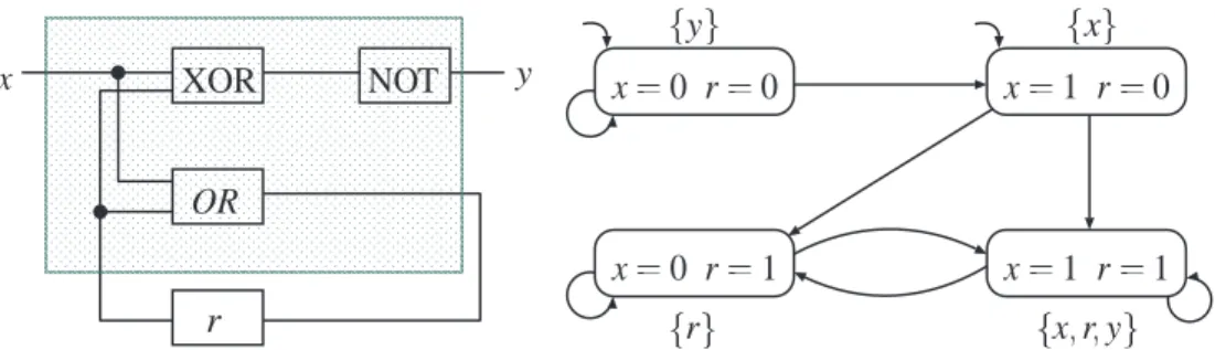
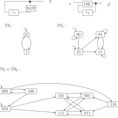
The theorems in AP are sufficient to formalize, e.g. the property "the output bit y is set infinitely often". Even if in real computer systems all domains are finite (eg the type integer includes only integers of a finite domain, such as -216< n <216), then the logical or algorithmic structure of a program is often based on infinite domains .
Program Graph (PG)
The nodes of a program graph are called locations and have a control function since they specify which of the conditional transitions are possible. Its states consist of a control component, i.e., a location of the program graph, together with an estimate η of the variables.
Transition System Semantics of a Program Graph The transition system TS(PG) of program graph
- Parallelism and Communication
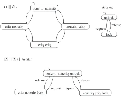
- Concurrency and Interleaving
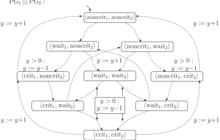
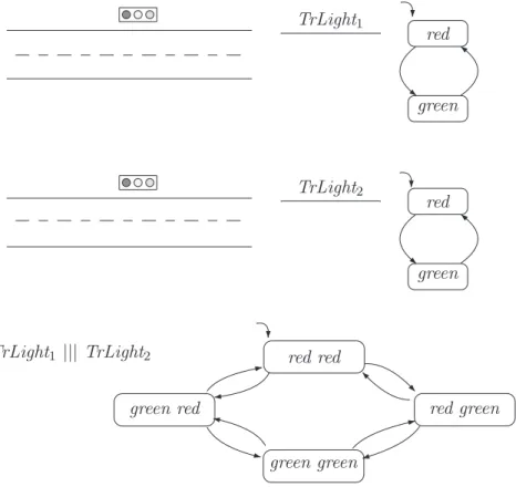
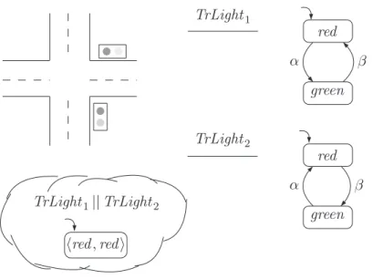
The transition system of the parallel assembly of both traffic lights is sketched at the bottom of Figure 2.4 where ||| denotes the interleaving operator. In principle, any form of interlocking of the "actions" of the two traffic lights is possible.
Interleaving of Transition Systems
- Communication via Shared Variables
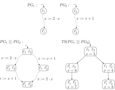
For dependent operations, the order of operations is typically significant: for example, the final value of variable x in the parallel program x := x+1|||x := 2·x (with the initial value x=0, for example) depends on the order in which the tasks x:=x+1 andx:= 2·x take place. For program graphs PG1 (on Var1) and PG2 (on Var2) without shared variables (i.e. Var1∩Var2=∅), the interleaving operator gives, which is applied to the appropriate transition systems, a transition system. that describes the behavior of the simultaneous execution of PG1 and PG2.
Interleaving of Program Graphs
- Handshaking
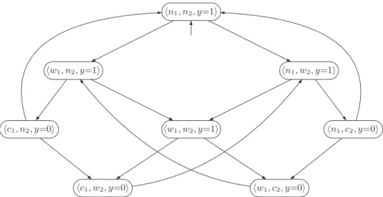
To model a parallel system using the interleaving operator for program graphs, it is crucial that the actionsα∈Actare are indivisible. As a result, both processes are simultaneously in their critical section and mutual exclusion is violated.
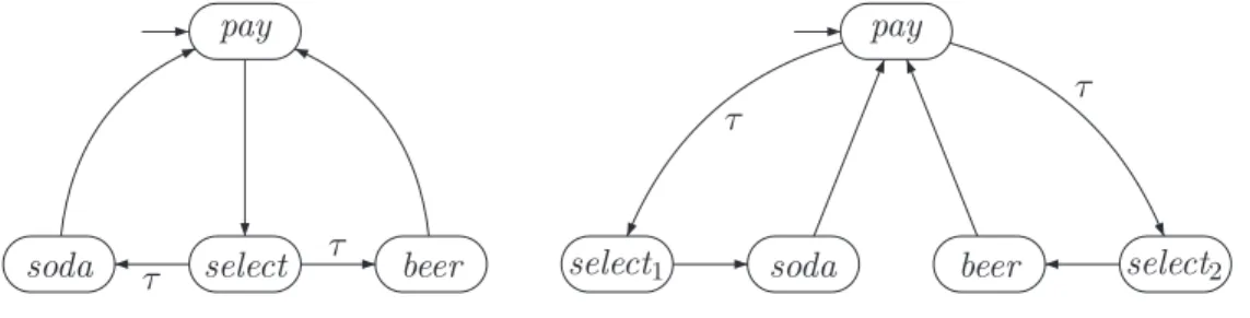
Handshaking (Synchronous Message Passing)
- Channel Systems
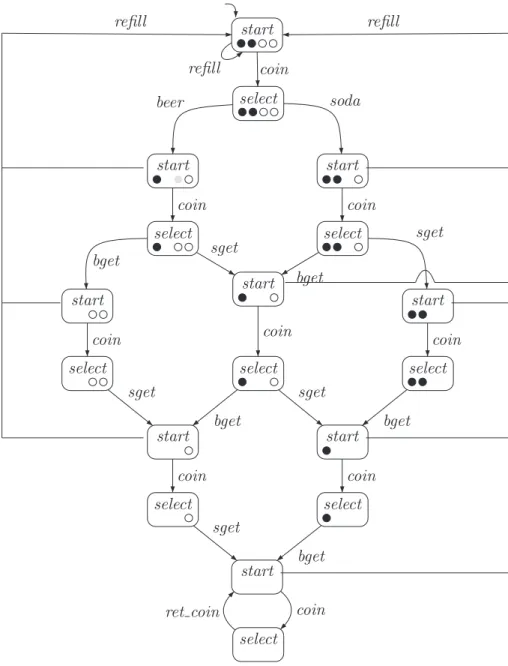
When the set H of handshake actions is empty, all actions of the participating processes can take place autonomously, i.e. in this special case handshaking is reduced to interleaving. The barcode reader reads a barcode and communicates the data of the product that has just been scanned to the booking program.
Channel System A program graph over (Var, Chan) is a tuple
- NanoPromela
This depends on the current variable evaluation and the capacity and content of the channel. Upon receiving m, b (along channel c), R sends an acknowledgment (ack) consisting of the just received control bit b.

Substatement
- Synchronous Parallelism
Pn] where the behavior of the process Pi is specified by a nanoPromela statement is a channel system [PG1|. The semantics of the atomic theorem skip is given by a single axiom that formalizes that the execution of skip ends in one step without affecting the variables.
Synchronous Product
- The State-Space Explosion Problem
- Summary
- Bibliographic Notes
- Exercises
The size of the transient system thus grows exponentially in the number of registers and input variables. Furthermore, the variables (and their domains) represented in the transient system significantly affect the size of the state space.
Linear-Time Properties
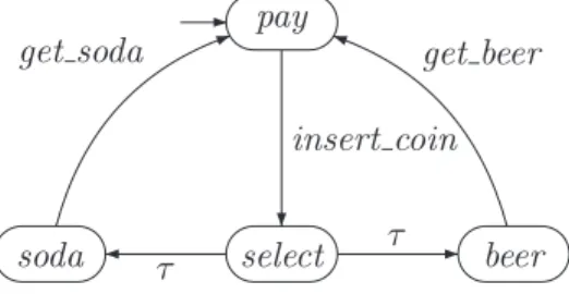
Deadlock
The deadlock situation mentioned above can be avoided by the fact that some sticks (eg the first, third and fifth stick) start in the availablei,i state, while the other sticks start in the availablei,i+1 state. In the case of the dining philosophers, robustness can be formulated to guarantee deadlock and famine, even if one of the philosophers is.
Linear-Time Behavior
State Graph
Path Fragment
Maximal and Initial Path Fragment
Path
- Traces
Recall that the tracks of a transition system have been defined as the tracks induced by its initial maximum path fragments. 3 A further alternative is to fit the linear time frame for transient systems with terminal states.
Trace and Trace Fragment
- Linear-Time Properties
Informally speaking, one could say that the property of linear time determines the permissible (or desired) behavior of the system under consideration. This definition is quite elementary and gives a good basic understanding of what a property of linear time is.

LT Property
Chapter 5 will present a logical formalism that enables the specification of linear time properties. Such a property can be understood as a requirement over all words over AP and is defined as the set of words (over AP) that are admissible:.
Satisfaction Relation for LT Properties
- Trace Equivalence and Linear-Time Properties
Let TS and TS be transitional systems with no final states and with the same set of propositions AP. Transitional systems are said to be trace equivalent if they have the same set of traces:.

Trace Equivalence
- Safety Properties and Invariants
- Invariants
Let TS and TS be transition systems without terminal states and with the same set of atomic numbers. Put another way, this means that there is no LT property that distinguishes between the two vending machines.
Invariant
- Safety Properties
For the locked-in freedom of the eating philosophers, the invariant ensures that at least one of the philosophers does not wait to pick up the chopstick. Safety Properties and Invariants 111 The worst-case time complexity of the proposed invariance checking algorithm is dominated by the cost of DFS visiting all available states.
Safety Properties, Bad Prefixes
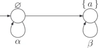
The minimum bad prefixes of this security property are regular in the sense that they constitute a regular language. The finite automaton in Figure 3-9 accepts exactly the minimum bad prefixes for the security property above.7 Here ¬yellow should be read as ∅ or {red}.

Prefix and Closure
- Trace Equivalence and Safety Properties
- Liveness Properties
Since this is usually undesirable, safety properties are supplemented with properties that require some progress. This is in contrast to safety properties where it is sufficient to have one finite trace (the "bad prefix") to conclude that a safety property is disproved.

Liveness Property
- Safety vs. Liveness Properties
- Fairness
The only LT property above AP that is both a safety and a vividness property is (2AP)ω. In the sequel, we adopt the action-based view and define strong justice for (series of) actions. In Chapter 5, state-based notions of justice will also be introduced and the relationship between action-based and state-based justice will be studied in detail.) Let A be a series of actions.

Unconditional, Strong, and Weak Fairness
The execution fragmentρ is strongly called A-fair if the actions in A are not continuously ignored under the condition that they can be executed infinitely many times. For example, an execution fragment that visits only states where no A-actions are possible is strong A-fair (since the premise of strong A-fair does not hold), but not unconditionally A-fair.
Fairness Assumption A fairness assumption for Act is a triple
As before, the reqi, enteri, and rel actions are used to model the request to enter the critical section, the entry itself, and the release of the critical section. Behavior in which one process has access to the critical section infinitely often while the other only gets access infinitely many times is very fair under this assumption.
Fair Satisfaction Relation for LT Properties
- Fairness and Safety
To force a synchronization to occur every now and then, the strong fairness assumption. Imposing the unconditional fairness assumption {{set}} ensures that the values 0 and 1 are executed infinitely often.
Realizable Fairness Assumption
- Summary
- Bibliographic Notes
- Exercises
Fairness 139 As an example of another form of fairness, consider the following sequential hardware circuit. The following theorem shows the irrelevance of realizable fairness assumptions for verifying security properties.
Regular Properties
Automata on Finite Words
Nondeterministic Finite Automaton (NFA)
Intuitively, q−−→A q indicates that the automaton can move from state q to state q when it reads the input symbol A. Finite automaton example. After reading the input symbol, the automaton changes its state according to the transition relationδ.
Runs, Accepted Language of an NFA
An NFA cannot perform any transition when its current state q does not have an outgoing transition labeled with the current input symbol A. Therefore, the class of regular languages corresponds to the class of languages accepted by an NFA.
Equivalence of NFAs
Regular languages exhibit some interesting closure properties, e.g. the merging of two common languages is correct. This follows directly from the definition of regular languages as those languages that can be generated using regular expressions.
Synchronous Product of NFAs
They are also closed under intersection and complementation, i.e. if L, L1, L2 are regular languages over the alphabet Σ, then so are L= Σ∗\ L and L1∩ L2. In both cases we can assume finite automata and assume a representation of the given regular languages by NFA A, A1 and A2 with the input alphabet Σ accepting the regular languages L, L1 and L2 respectively.
Deterministic Finite Automaton (DFA)
- Model-Checking Regular Safety Properties
- Regular Safety Properties
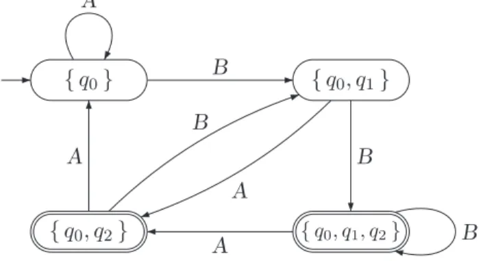
An intuitive argument for the latter is that any DFA for L(Ek) must "remember" the Ba symbol positions among the last input symbols, yielding Ω(2k) states. The main result of this section is that checking the regular security property on a finite transitive system can be reduced to an invariant check of the product TS and NFA A for bad prefixes.
Regular Safety Property
- Verifying Regular Safety Properties
- Automata on Infinite Words
- ω -Regular Languages and Properties
- Nondeterministic B¨ uchi Automata
The language of minimum bad prefixes safety features “every red light phase. The intuitive meaning of the acceptance criterion, named after B¨uchi, is that the acceptable set A (ie, the set of acceptable states in A) must be visited infinitely often.

Nondeterministic B¨ uchi Automaton (NBA)
The accepting executions of an ω-automata must "check" the entire input word (and not just a finite prefix of it), and thus must be infinite. Automaton A is in the acceptance state q1 if and only if the last input set of symbols (i.e., the last setAi) contains the green propositional symbol.


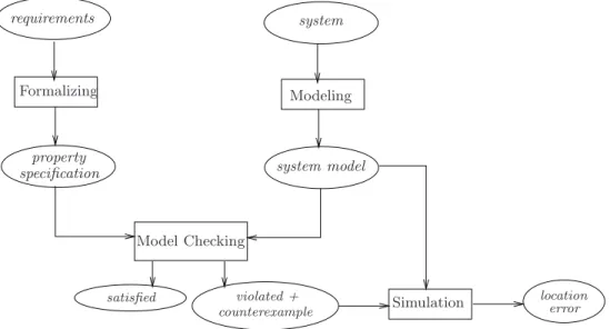
![Figure 1.3: Software lifecycle and error introduction, detection, and repair costs [275].](https://thumb-ap.123doks.com/thumbv2/123dok/9604779.0/24.864.226.643.100.316/figure-software-lifecycle-error-introduction-detection-repair-costs.webp)