Biostatistics for Animal Science
Miroslav Kaps
University of Zagreb, Croatiaand
William R. Lamberson
University of Missouri-Columbia, USACABI Publishing
CABI Publishing CAB International Wallingford
Oxfordshire OX10 8DE UK
Tel: +44 (0)1491 832111 Fax: +44 (0)1491 833508 E-mail: [email protected]
Web site: www.cabi-publishing.org
CABI Publishing 875 Massachusetts Avenue
7th Floor Cambridge, MA 02139 USA Tel: +1 617 395 4056 Fax: +1 617 354 6875 E-mail: [email protected]
© M. Kaps and W.R. Lamberson 2004. All rights reserved. No part of this publication may be reproduced in any form or by any means, electronically, mechanically, by photocopying, recording or otherwise, without the prior permission of the copyright owners. ‘ All queries to be referred to the publisher.
A catalogue record for this book is available from the British Library, London, UK.
Library of Congress Cataloging-in-Publication Data Kaps, Miroslav
Biostatistics for animal science / by Miroslav Kaps and William R Lamberson.
p. cm.
Includes bibliographical references and index.
ISBN 0-85199-820-8 (alk. paper)
1. Livestock--Statistical methods. 2. Biometry. I. Lamberson, William R. II. Title.
SF140.S72K37 2004 636’.007’27--dc22
2004008002
ISBN 0 85199 820 8
Printed and bound in the UK by Cromwell Press, Trowbridge, from copy supplied by the authors
v PREFACE XII
CHAPTER 1 PRESENTING AND SUMMARIZING DATA ... 1
1.1 DATA AND VARIABLES...1
1.2 GRAPHICAL PRESENTATION OF QUALITATIVE DATA ...2
1.3 GRAPHICAL PRESENTATION OF QUANTITATIVE DATA ...3
1.3.1 Construction of a Histogram ...3
1.4 NUMERICAL METHODS FOR PRESENTING DATA...6
1.4.1 Symbolic Notation ...6
1.4.2 Measures of Central Tendency...7
1.4.3 Measures of Variability...8
1.4.4 Measures of the Shape of a Distribution ...9
1.4.5 Measures of Relative Position...11
1.5 SAS EXAMPLE ...12
EXERCISES ...13
CHAPTER 2 PROBABILITY ... 15
2.1 RULES ABOUT PROBABILITIES OF SIMPLE EVENTS ...15
2.2 COUNTING RULES ...16
2.2.1 Multiplicative Rule...17
2.2.2 Permutations...17
2.2.3 Combinations ...18
2.2.4 Partition Rule ...18
2.2.5 Tree Diagram ...18
2.3 COMPOUND EVENTS...19
2.4 BAYES THEOREM ...23
EXERCISES ...25
CHAPTER 3 RANDOM VARIABLES AND THEIR DISTRIBUTIONS ... 26
3.1 EXPECTATIONS AND VARIANCES OF RANDOM VARIABLES ...26
3.2 PROBABILITY DISTRIBUTIONS FOR DISCRETE RANDOM VARIABLES ..28
3.2.1 Expectation and Variance of a Discrete Random Variable ...29
3.2.2 Bernoulli Distribution ...30
3.2.3 Binomial Distribution...31
3.2.4 Hyper-geometric Distribution ...33
3.2.5 Poisson Distribution ...34
3.2.6 Multinomial Distribution...35
3.3 PROBABILITY DISTRIBUTIONS FOR CONTINUOUS RANDOM VARIABLES...36
3.3.1 Uniform Distribution...37
3.3.2 Normal Distribution ...37
3.3.3 Multivariate Normal Distribution...45
3.3.4 Chi-square Distribution...47
3.3.5 Student t Distribution ...48
3.3.6 F Distribution ...50
EXERCISES ...51
CHAPTER 4 POPULATION AND SAMPLE ... 53
4.1 FUNCTIONS OF RANDOM VARIABLES AND SAMPLING DISTRIBUTIONS ...53
4.1.1 Central Limit Theorem...54
4.1.2 Statistics with Distributions Other than Normal ...54
4.2 DEGREES OF FREEDOM...55
CHAPTER 5 ESTIMATION OF PARAMETERS... 56
5.1 POINT ESTIMATION ...56
5.2 MAXIMUM LIKELIHOOD ESTIMATION ...57
5.3 INTERVAL ESTIMATION ...58
5.4 ESTIMATION OF PARAMETERS OF A NORMAL POPULATION...60
5.4.1 Maximum Likelihood Estimation ...60
5.4.2 Interval Estimation of the Mean...61
5.4.3 Interval Estimation of the Variance...62
EXERCISES ...64
CHAPTER 6 HYPOTHESIS TESTING... 65
6.1 HYPOTHESIS TEST OF A POPULATION MEAN ...66
6.1.1 P value...69
6.1.2 A Hypothesis Test Can Be One- or Two-sided...70
6.1.3 Hypothesis Test of a Population Mean for a Small Sample...71
6.2 HYPOTHESIS TEST OF THE DIFFERENCE BETWEEN TWO POPULATION MEANS...72
6.2.1 Large Samples...72
6.2.2 Small Samples and Equal Variances ...74
6.2.3 Small Samples and Unequal Variances...75
6.2.4 Dependent Samples...75
6.2.5 Nonparametric Test...76
6.2.6 SAS Examples for Hypotheses Tests of Two Population Means...79
6.3 HYPOTHESIS TEST OF A POPULATION PROPORTION...81
6.4 HYPOTHESIS TEST OF THE DIFFERENCE BETWEEN PROPORTIONS FROM TWO POPULATIONS ...82
6.5 CHI-SQUARE TEST OF THE DIFFERENCE BETWEEN OBSERVED AND EXPECTED FREQUENCIES ...84
6.5.1 SAS Example for Testing the Difference between Observed and Expected Frequencies ...85
6.6 HYPOTHESIS TEST OF DIFFERENCES AMONG PROPORTIONS FROM SEVERAL POPULATIONS ...86
6.6.1 SAS Example for Testing Differences among Proportions from Several Populations...88
6.7 HYPOTHESIS TEST OF POPULATION VARIANCE ...90
6.8 HYPOTHESIS TEST OF THE DIFFERENCE OF TWO POPULATION VARIANCES...90
6.9 HYPOTHESIS TESTS USING CONFIDENCE INTERVALS ...91
6.10 STATISTICAL AND PRACTICAL SIGNIFICANCE...92
6.11 TYPES OF ERRORS IN INFERENCES AND POWER OF TEST ...92
6.11.1 SAS Examples for the Power of Test...99
6.12 SAMPLE SIZE ...103
6.12.1 SAS Examples for Sample Size ...104
EXERCISES ...107
CHAPTER 7 SIMPLE LINEAR REGRESSION ... 109
7.1 THE SIMPLE REGRESSION MODEL ...109
7.2 ESTIMATION OF THE REGRESSION PARAMETERS – LEAST SQUARES ESTIMATION ...113
7.3 MAXIMUM LIKELIHOOD ESTIMATION ...116
7.4 RESIDUALS AND THEIR PROPERTIES...117
7.5 EXPECTATIONS AND VARIANCES OF THE PARAMETER ESTIMATORS...119
7.6 STUDENT T TEST IN TESTING HYPOTHESES ABOUT THE PARAMETERS...120
7.7 CONFIDENCE INTERVALS OF THE PARAMETERS ...121
7.8 MEAN AND PREDICTION CONFIDENCE INTERVALS OF THE RESPONSE VARIABLE ...122
7.9 PARTITIONING TOTAL VARIABILITY...124
7.9.1 Relationships among Sums of Squares ...126
7.9.2 Theoretical Distribution of Sum of Squares...127
7.10 TEST OF HYPOTHESES - F TEST ...128
7.11 LIKELIHOOD RATIO TEST...130
7.12 COEFFICIENT OF DETERMINATION ...132
7.12.1 Shortcut Calculation of Sums of Squares and the Coefficient of Determination...133
7.13 MATRIX APPROACH TO SIMPLE LINEAR REGRESSION ...134
7.13.1 The Simple Regression Model ...134
7.13.2 Estimation of Parameters ...135
7.13.3 Maximum Likelihood Estimation ...138
7.14 SAS EXAMPLE FOR SIMPLE LINEAR REGRESSION ...139
7.15 POWER OF TESTS...140
7.15.1 SAS Examples for Calculating the Power of Test ...142
EXERCISES ...144
CHAPTER 8 CORRELATION... 146
8.1 ESTIMATION OF THE COEFFICIENT OF CORRELATION AND TESTS OF HYPOTHESES ...147
8.2 NUMERICAL RELATIONSHIP BETWEEN THE SAMPLE COEFFICIENT OF CORRELATION AND THE COEFFICIENT OF DETERMINATION...149
8.2.1 SAS Example for Correlation ...150
8.3 RANK CORRELATION ...151
8.3.1 SAS Example for Rank Correlation ...152
EXERCISES ...153
CHAPTER 9 MULTIPLE LINEAR REGRESSION... 154
9.1 TWO INDEPENDENT VARIABLES ...155
9.1.1 Estimation of Parameters ...156
9.1.2 Student t test in Testing Hypotheses ...159
9.1.3 Partitioning Total Variability and Tests of Hypotheses ...160
9.2 PARTIAL AND SEQUENTIAL SUMS OF SQUARES ...162
9.3 TESTING MODEL FIT USING A LIKELIHOOD RATIO TEST...166
9.4 SAS EXAMPLE FOR MULTIPLE REGRESSION...168
9.5 POWER OF MULTIPLE REGRESSION ...170
9.5.1 SAS Example for Calculating Power ...171
9.6 PROBLEMS WITH REGRESSION...172
9.6.1 Analysis of Residuals...173
9.6.2 Extreme Observations ...174
9.6.3 Multicollinearity...177
9.6.4 SAS Example for Detecting Problems with Regression ...178
9.7 CHOOSING THE BEST MODEL ...181
9.7.1 SAS Example for Model Selection ...183
CHAPTER 10CURVILINEAR REGRESSION ... 185
10.1 POLYNOMIAL REGRESSION...185
10.1.1 SAS Example for Quadratic Regression ...189
10.2 NONLINEAR REGRESSION...190
10.2.1 SAS Example for Nonlinear Regression...192
10.3 SEGMENTED REGRESSION...194
10.3.1 SAS Examples for Segmented Regression...198
10.3.1.1 SAS Example for Segmented Regression with Two Simple Regressions...198
10.3.1.2 SAS Example for Segmented Regression with Plateau ...200
CHAPTER 11ONE-WAY ANALYSIS OF VARIANCE ... 204
11.1 THE FIXED EFFECTS ONE-WAY MODEL ...206
11.1.1 Partitioning Total Variability ...208
11.1.2 Hypothesis Test - F Test ...210
11.1.3 Estimation of Group Means ...214
11.1.4 Maximum Likelihood Estimation ...214
11.1.5 Likelihood Ratio Test...215
11.1.6 Multiple Comparisons among Group Means ...217
11.1.6.1 Least Significance Difference (LSD)...217
11.1.6.2 Tukey Test...218
11.1.6.3 Contrasts ...220
11.1.6.4 Orthogonal contrasts ...221
11.1.6.5 Scheffe Test...223
11.1.7 Test of Homogeneity of Variance ...225
11.1.8 SAS Example for the Fixed Effects One-way Model ...226
11.1.9 Power of the Fixed Effects One-way Model...228
11.1.9.1 SAS Example for Calculating Power ...230
11.2 THE RANDOM EFFECTS ONE-WAY MODEL ...231
11.2.1 Hypothesis Test...233
11.2.2 Prediction of Group Means ...234
11.2.3 Variance Component Estimation...235
11.2.4 Intraclass Correlation ...237
11.2.5 Maximum Likelihood Estimation ...238
11.2.6 Restricted Maximum Likelihood Estimation ...240
11.2.7 SAS Example for the Random Effects One-way Model ...241
11.3 MATRIX APPROACH TO THE ONE-WAY ANALYSIS OF VARIANCE MODEL ...243
11.3.1 The Fixed Effects Model...243
11.3.1.1 Linear Model...243
11.3.1.2 Estimating Parameters...245
11.3.1.3 Maximum Likelihood Estimation ...249
11.3.1.4 Regression Model for the One-way Analysis of Variance...250
11.3.2 The Random Effects Model ...253
11.3.2.1 Linear Model...253
11.3.2.2 Prediction of Random Effects...254
11.3.2.3 Maximum Likelihood Estimation ...256
11.3.2.4 Restricted Maximum Likelihood Estimation ...257
11.4 MIXED MODELS ...257
11.4.1.1 Prediction of Random Effects...258
11.4.1.2 Maximum Likelihood Estimation ...259
11.4.1.3 Restricted Maximum Likelihood Estimation ...260
EXERCISES ...262
CHAPTER 12CONCEPTS OF EXPERIMENTAL DESIGN... 263
12.1 EXPERIMENTAL UNITS AND REPLICATIONS ...264
12.2 EXPERIMENTAL ERROR...265
12.3 PRECISION OF EXPERIMENTAL DESIGN...266
12.4 CONTROLLING EXPERIMENTAL ERROR...268
12.5 REQUIRED NUMBER OF REPLICATIONS ...269
12.5.1 SAS Example for the Number of Replications ...270
CHAPTER 13BLOCKING ... 272
13.1 RANDOMIZED COMPLETE BLOCK DESIGN...272
13.1.1 Partitioning Total Variability ...274
13.1.2 Hypotheses Test - F test...275
13.1.3 SAS Example for Block Design...279
13.2 RANDOMIZED BLOCK DESIGN – TWO OR MORE UNITS PER TREATMENT AND BLOCK ...280
13.2.1 Partitioning Total Variability and Test of Hypotheses...281
13.2.2 SAS Example for Two or More Experimental Unit per Block x Treatment...287
13.3 POWER OF TEST ...291
13.3.1 SAS Example for Calculating Power ...291
EXERCISES ...293
CHAPTER 14CHANGE-OVER DESIGNS... 294
14.1 SIMPLE CHANGE-OVER DESIGN ...294
14.2 CHANGE-OVER DESIGNS WITH THE EFFECTS OF PERIODS...297
14.2.1 SAS Example for Change-over Designs with the Effects of Periods...299
14.3 LATIN SQUARE...301
14.3.1 SAS Example for Latin Square ...305
14.4 CHANGE-OVER DESIGN SET AS SEVERAL LATIN SQUARES ...307
14.4.1 SAS Example for Several Latin Squares...309
EXERCISES ...311
CHAPTER 15FACTORIAL EXPERIMENTS... 313
15.1 THE TWO FACTOR FACTORIAL EXPERIMENT...313
15.2 SAS EXAMPLE FOR FACTORIAL EXPERIMENT ...320
EXERCISE ...322
CHAPTER 16HIERARCHICAL OR NESTED DESIGN... 323
16.1 HIERARCHICAL DESIGN WITH TWO FACTORS...323
16.2 SAS EXAMPLE FOR HIERARCHICAL DESIGN ...328
CHAPTER 17MORE ABOUT BLOCKING... 331
17.1 BLOCKING WITH PENS, CORRALS AND PADDOCKS ...331
17.1.1 SAS Example for Designs with Pens and Paddocks ...334
17.2 DOUBLE BLOCKING...338
CHAPTER 18SPLIT-PLOT DESIGN ... 342
18.1 SPLIT-PLOT DESIGN – MAIN PLOTS IN RANDOMIZED BLOCKS...342
18.1.1 SAS Example: Main Plots in Randomized Blocks...346
18.2 SPLIT-PLOT DESIGN – MAIN PLOTS IN A COMPLETELY RANDOMIZED DESIGN...348
18.2.1 SAS Example: Main Plots in a Completely Randomized Design ...351
EXERCISE ...354
CHAPTER 19ANALYSIS OF COVARIANCE ... 355
19.1 COMPLETELY RANDOMIZED DESIGN WITH A COVARIATE...355
19.1.1 SAS Example for a Completely Randomized Design with a Covariate...356
19.2 TESTING THE DIFFERENCE BETWEEN REGRESSION SLOPES ...358
19.2.1 SAS Example for Testing the Difference between Regression Slopes ...363
CHAPTER 20REPEATED MEASURES ... 365
20.1 HOMOGENEOUS VARIANCES AND COVARIANCES AMONG REPEATED MEASURES ...365
20.1.1 SAS Example for Homogeneous Variances and Covariances ...368
20.2 HETEROGENEOUS VARIANCES AND COVARIANCES AMONG REPEATED MEASURES ...372
20.2.1 SAS Examples for Heterogeneous Variances and Covariances...373
20.3 RANDOM COEFFICIENT REGRESSION...376
20.3.1 SAS Examples for Random Coefficient Regression ...377
20.3.1.1 Homogeneous Variance-Covariance Parameters across Treatments ...377
20.3.1.2 Heterogeneous Variance-Covariance Parameters across Treatments ...379
CHAPTER 21ANALYSIS OF NUMERICAL TREATMENT LEVELS... 384
21.1 LACK OF FIT...384
21.1.1 SAS Example for Lack of Fit...387
21.2 POLYNOMIAL ORTHOGONAL CONTRASTS ...389
21.2.1 SAS Example for Polynomial Contrasts ...391
CHAPTER 22DISCRETE DEPENDENT VARIABLES ... 394
22.1 LOGIT MODELS, LOGISTIC REGRESSION...395
22.1.1 Testing Hypotheses ...397
22.1.2 SAS Examples for Logistic Models ...402
22.2 PROBIT MODEL ...407
22.2.1 SAS Example for a Probit model ...409
22.3 LOG-LINEAR MODELS ...412
22.3.1 SAS Example for a Log-Linear Model ...415
SOLUTIONS OF EXERCISES... 419
APPENDIX A: VECTORS AND MATRICES... 421
TYPES AND PROPERTIES OF MATRICES ...421
MATRIX AND VECTOR OPERATIONS ...422
APPENDIX B: STATISTICAL TABLES... 426
AREA UNDER THE STANDARD NORMAL CURVE, Z > Zα...426
CRITICAL VALUES OF STUDENT T DISTRIBUTIONS, T > Tα...427
CRITICAL VALUES OF CHI-SQUARE DISTRIBUTIONS, χ2 > χ2α...429
CRITICAL VALUES OF F DISTRIBUTIONS, F > Fα, α = 0.05 ...431
CRITICAL VALUE OF F DISTRIBUTIONS, F > Fα, α = 0.01...433
CRITICAL VALUES OF THE STUDENTIZED RANGE, Q(A,V) ...435
REFERENCES... 436
SUBJECT INDEX... 439
xii
This book was written to serve students and researchers of the animal sciences, with the primary purpose of helping them to learn about and apply appropriate experimental designs and statistical methods. Statistical methods applied to biological sciences are known as biostatistics or biometrics, and they have their origins in agricultural research. The characteristic that distinguishes biometrics within statistics is the fact that biological measurements are variable, not only because of measurement error, but also from their natural variability from genetic and environmental sources. These sources of variability must be taken into account when making inferences about biological material. Accounting for these sources of variation has led to the development of experimental designs that incorporate blocking, covariates and repeated measures. Appropriate techniques for analysis of data from these designs and others are covered in the book.
Early in the book, readers are presented basic principles of statistics so they will be able to follow subsequent applications with familiarity and understanding, and without having to switch to another book of introductory statistics. Later chapters cover statistical methods most frequently used in the animal sciences for analysis of continuous and categorical variables. Each chapter begins by introducing a problem with practical questions, followed with a brief theoretical background and short proofs. The text is augmented with examples, mostly from animal sciences and related fields, with the purpose of making applications of the statistical methods familiar. Some examples are very simple and are presented in order to provide basic understanding and the logic behind calculations.
These examples can be solved using a pocket calculator. Some examples are more complex, especially those in the later chapters. Most examples are also solved using SAS statistical software. Both sample SAS programs and SAS listings are given with brief explanations.
Further, the solutions are often given with sufficient decimal digits, more than is practically necessary, so that readers can compare results to verify calculation technique.
The first five chapters of the book are: 1) Presenting and Summarizing Data; 2) Probability; 3) Random Variables and Their Distributions; 4) Population and Sample; and 5) Estimation of Parameters. These chapters provide a basic introduction to biostatistics including definitions of terms, coverage of descriptive statistics and graphical presentation of data, the basic rules of probability, methods of parameter estimation, and descriptions of distributions including the Bernoulli, binomial, hypergeometric, Poisson, multinomial, uniform, normal, chi-square, t, and F distributions. Chapter 6 describes hypothesis testing and includes explanations of the null and alternate hypotheses, use of probability or density functions, critical values, critical region and P values. Hypothesis tests for many specific cases are shown such as population means and proportions, expected and empirical frequency, and test of variances. Also, the use of confidence intervals in hypothesis testing is shown. The difference between statistical and practical significance, types of errors in making conclusions, power of test, and sample size are discussed.
Chapters 7 to 10 present the topics of correlation and regression. The coverage begins with simple linear regression and describes the model, its parameters and assumptions.
Least squares and maximum likelihood methods of parameter estimation are shown. The concept of partitioning the total variance to explained and unexplained sources in the analysis of variance table is introduced. In chapter 8 the general meaning and definition of
the correlation coefficient, and the estimation of the correlation coefficient from samples and testing of hypothesis are shown. In chapters 9 and 10 multiple and curvilinear regressions are described. Important facts are explained using matrices in the same order of argument as for the simple regression. Model building is introduced including the definitions of partial and sequential sum of squares, test of model adequacy using a likelihood function, and Conceptual Predictive and Akaike criteria. Some common problems of regression analysis like outliers and multicollinearity are described, and their detection and possible remedies are explained. Polynomial, nonlinear and segmented regressions are introduced. Some examples are shown including estimating growth curves and functions with a plateau such as for determining nutrient requirements.
One-way analysis of variance is introduced in chapter 11. In this chapter a one-way analysis of variance model is used to define hypotheses, partition sums of squares in order to use an F test, and estimate means and effects. Post-test comparison of means, including least significant difference, Tukey test and contrasts are shown. Fixed and random effects models are compared, and fixed and random effects are also shown using matrices.
Chapters 12 to 21 focus on specific experimental designs and their analyses. Specific topics include: general concepts of design, blocking, change-over designs, factorials, nested designs, double blocking, split-plots, analysis of covariance, repeated measures and analysis of numerical treatment levels. Examples with sample SAS programs are provided for each topic.
The final chapter covers the special topic of discrete dependent variables. Logit and probit models for binary and binomial dependent variables and loglinear models for count data are explained. A brief theoretical background is given with examples and SAS procedures.
We wish to express our gratitude to everyone who helped us produce this book. We extend our special acknowledgement to Matt Lucy, Duane Keisler, Henry Mesa, Kristi Cammack, Marijan Posavi and Vesna Luzar-Stiffler for their reviews, and Cyndi Jennings, Cinda Hudlow and Dragan Tupajic for their assistance with editing.
Zagreb, Croatia Miroslav Kaps
Columbia, Missouri William R. Lamberson
March 2004
1
Chapter 1
Presenting and Summarizing Data
1.1 Data and Variables
Data are the material with which statisticians work. They are records of measurement, counts or observations. Examples of data are records of weights of calves, milk yield in lactation of a group of cows, male or female sex, and blue or green color of eyes. A set of observations on a particular character is termed a variable. For example, variables denoting the data listed above are weight, milk yield, sex, and eye color. Data are the values of a variable, for example, a weight of 200 kg, a daily milk yield of 20 kg, male, or blue eyes.
The expression variable depicts that measurements or observations can be different, i.e., they show variability. Variables can be defined as quantitative (numerical) and qualitative (attributive, categorical, or classification).
Quantitative variables have values expressed as numbers and the differences between values have numerical meaning. Examples of quantitative variables are weight of animals, litter size, temperature or time. They also can include ratios of two numerical variables, count data, and proportions. A quantitative variable can be continuous or discrete. A continuous variable can take on an infinite number of values over a given interval. Its values are real numbers. A discrete variable is a variable that has countable values, and the number of those values can either be finite or infinite. Its values are natural numbers or integers.
Examples of continuous variables are milk yield or weight, and examples of discrete variables are litter size or number of laid eggs per month.
Qualitative variables have values expressed in categories. Examples of qualitative variables are eye color or whether or not an animal is ill. A qualitative variable can be an ordinal or nominal. An ordinal variable has categories that can be ranked. A nominal variable has categories that cannot be ranked. No category is more valuable than another.
Examples of nominal variables are identification number, color or gender, and an example of an ordinal variable is calving ease scoring. For example, calving ease can be described in 5 categories, but those categories can be enumerated: 1. normal calving, 2. calving with little intervention, 3. calving with considerable intervention, 4. very difficult calving, and 5.
Caesarean section. We can assign numbers (scores) to ordinal categories; however, the differences among those numbers do not have numerical meaning. For example, for calving ease, the difference between score 1 and 2 (normal calving and calving with little intervention) does not have the same meaning as the difference between 4 and 5 (very difficult calving and Caesarean section). As a rule those scores depict categories, but not a numerical scale. On the basis of the definition of a qualitative variable it may be possible to assign some quantitative variables, for example, the number of animals that belong to a category, or the proportion of animals in one category out of the total number of animals.
1.2 Graphical Presentation of Qualitative Data
When describing qualitative data each observation is assigned to a specific category. Data are then described by the number of observations in each category or by the proportion of the total number of observations. The frequency for a certain category is the number of observations in that category. The relative frequency for a certain category is the proportion of the total number of observations. Graphical presentations of qualitative variables can include bar, column or pie-charts.
Example: The numbers of cows in Croatia under milk recording by breed are listed in the following table:
Breed Number of cows Percentage
Simmental 62672 76%
Holstein-Friesian 15195 19%
Brown 3855 5%
Total 81722 100%
The number of cows can be presented using bars with each bar representing a breed (Figure 1.1).
62672 15195
3855
0 20000 40000 60000 80000
Simmental Holstein Brown
Breed
Number of cows
Figure 1.1 Number of cows under milk recording by breed
The proportions or percentage of cows by breed can also be shown using a pie-chart (Figure 1.2).
Simmental 76%
Holstein 19%
Brown 5%
Figure 1.2 Percentage of cows under milk recording by breed
1.3 Graphical Presentation of Quantitative Data
The most widely used graph for presentation of quantitative data is a histogram. A histogram is a frequency distribution of a set of data. In order to present a distribution, the quantitative data are partitioned into classes and the histogram shows the number or relative frequency of observations for each class.
1.3.1 Construction of a Histogram
Instructions for drawing a histogram can be listed in several steps:
1. Calculate the range: (Range = maximum – minimum value)
2. Divide the range into five to 20 classes, depending on the number of observations. The class width is obtained by rounding the result up to an integer number. The lowest class boundary must be defined below the minimum value, the highest class boundary must be defined above the maximum value.
3. For each class, count the number of observations belonging to that class. This is the true frequency.
4. The relative frequency is calculated by dividing the true frequency by the total number of observations: (Relative frequency = true frequency / total number of observations).
5. The histogram is a column (or bar) graph with class boundaries defined on one axis and frequencies on the other axis.
Example: Construct a histogram for the 7-month weights (kg) of 100 calves:
233 208 306 300 271 304 207 254 262 231 279 228 287 223 247 292 209 303 194 268 263 262 234 277 291 277 256 271 255 299 278 290 259 251 265 316 318 252 316 221 249 304 241 249 289 211 273 241 215 264 216 271 296 196 269 231 272 236 219 312 320 245 263 244 239 227 275 255 292 246 245 255 329 240 262 291 275 272 218 317 251 257 327 222 266 227 255 251 298 255 266 255 214 304 272 230 224 250 255 284 Minimum = 194
Maximum = 329 Range = 329 - 194 = 135
For a total 15 classes, the width of a class is:
135 / 15 = 9
The class width can be rounded to 10 and the following table constructed:
Class
limits Class
midrange Number of
calves Relative
Frequency (%) Cumulative number of calves
185 - 194 190 1 1 1
195 - 204 200 1 1 2
205 - 214 210 5 5 7
215 - 224 220 8 8 15
225 - 234 230 8 8 23
235 - 244 240 6 6 29
245 - 254 250 12 12 41
255 - 264 260 16 16 57
265 - 274 270 12 12 69
275 - 284 280 7 7 76
285 - 294 290 7 7 83
295 - 304 300 8 8 91
305 - 314 310 2 2 93
315 - 324 320 5 5 98
325 - 334 330 2 2 100
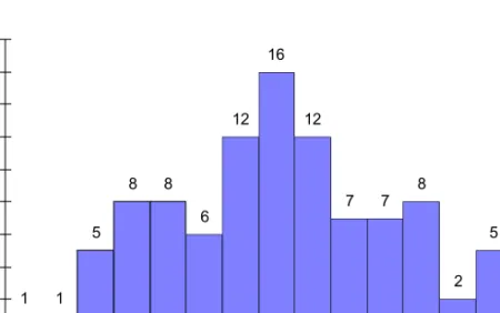
Figure 1.3 presents the histogram of weights of calves. The classes are on the horizontal axis and the numbers of animals are on the vertical axis. Class values are expressed as the class midranges (midpoint between the limits), but could alternatively be expressed as class limits.
1 1 5
8 8
6 12
16
12
7 7 8
2 5
2
0 2 4 6 8 10 12 14 16 18
190 200 210 220 230 240 250 260 270 280 290 300 310 320 330 Class midrange (kg)
Number of calves
Figure 1.3 Histogram of weights of calves at seven months of age (n=100)
Another well-known way of presenting quantitative data is by the use of a ‘Stem and Leaf’
graph. The construction of a stem and leaf can be shown in three steps:
1. Each value is divided into two parts, ‘Stem’ and ‘Leaf’. ‘Stem’ corresponds to higher decimal places, and ‘Leaf’ corresponds to lower decimal places. For the example of calf weights, the first two digits of each weight would represent the stem and the third digit the leaf.
2. ‘Stems’ are sorted in ascending order in the first column.
3. The appropriate ‘Leaf’ for each observation is recorded in the row with the appropriate ‘Stem’.
A ‘Stem and Leaf’ plot of the weights of calves is shown below.
Stem Leaf 19 | 4 6 20 | 7 8 9 21 | 1 4 5 6 8 9 22 | 1 2 3 4 7 8 23 | 0 1 1 3 4 6 9 24 | 0 1 1 4 5 5 6 7 9 9
25 | 0 1 1 1 2 4 5 5 5 5 5 5 5 6 7 9 26 | 2 2 2 3 3 4 5 6 6 8 9 27 | 1 1 1 2 2 2 3 5 5 7 7 8 9 28 | 4 7 9
29 | 0 1 1 2 2 6 8 9 30 | 0 3 4 4 4 6 31 | 2 6 6 7 8 32 | 0 7 9
For example, in the next to last row the ‘Stem’ is 31 and ‘Leaves’ are 2, 6, 6, 7 and 8. This indicates that the category includes the measurements 312, 316, 316, 317 and 318. When the data are suited to a stem and leaf plot it shows a distribution similar to the histogram and also shows each value of the data.
1.4 Numerical Methods for Presenting Data
Numerical methods for presenting data are often called descriptive statistics. They include:
a) measures of central tendency; b) measures of variability ; c) measures of the shape of a distribution; and d) measures of relative standing.
Descriptive statistics a) measures of
central tendency
b) measures of variability
c) measures of the shape of a
distribution
d) measures of relative position - arithmetic mean - range - skewness - percentiles
- median - variance - kurtosis - z-values
- mode - standard deviation - coefficient of
variation
Before descriptive statistics are explained in detail, it is useful to explain a system of symbolic notation that is used not only in descriptive statistics, but in statistics in general.
This includes the symbols for the sum, sum of squares and sum of products.
1.4.1 Symbolic Notation
The Greek letter
Σ
(sigma) is used as a symbol for summation, and yi for the value for observation i.The sum of n numbers y1, y2,…, yn can be expressed:
Σ
i yi = y1 + y2 +...+ ynThe sum of squares of n numbers y1, y2,…, yn is:
Σ
i y2i = y21 + y22 +...+ y2nThe sum of products of two sets of n numbers (x1, x2,…, xn) and (y1, y2,…, yn):
Σ
i xiyi = x1y1 + x2y2 +...+ xnynExample: Consider a set of three numbers: 1, 3 and 6. The numbers are symbolized by:
y1 = 1, y2 = 3 and y3 = 6.
The sum and sum of squares of those numbers are:
Σ
i yi = 1 + 3 + 6 = 10Σ
i y2i = 12 + 32 + 62 = 46Consider another set of numbers: x1 = 2, x2 = 4 and x3 = 5.
The sum of products of x and y is:
Σ
i xiyi = (1)(2) + (3)(4) + (6)(5) = 44 Three main rules of addition are:1. The sum of addition of two sets of numbers is equal to the addition of the sums:
Σ
i (xi + yi) =Σ
i xi +Σ
i yi2. The sum of products of a constant k and a variable y is equal to the product of the constant and the sum of the values of the variable:
Σ
i k yi = kΣ
i yi3. The sum of n constants with value k is equal to the product n k:
Σ
i k = n k1.4.2 Measures of Central Tendency
Commonly used measures of central tendency are the arithmetic mean, median and mode.
The arithmetic mean of a sample of n numbers y1,y2,..., yn is:
n y=
∑
iyiThe arithmetic mean for grouped data is:
n y y=
∑
ifi iwith fi being the frequency or proportion of observations yi. If fi is a proportion then n = 1.
Important properties of the arithmetic mean are:
1.
∑
i(
yi−y)
=0The sum of deviation from the arithmetic mean is equal to zero. This means that only (n - 1) observations are independent and the nth can be expressed as
1 1−...− −
−
= n
n ny y y
y
2.
∑
i(
yi−y)
2=minimumThe sum of squared deviations from the arithmetic mean is smaller than the sum of squared deviations from any other value.
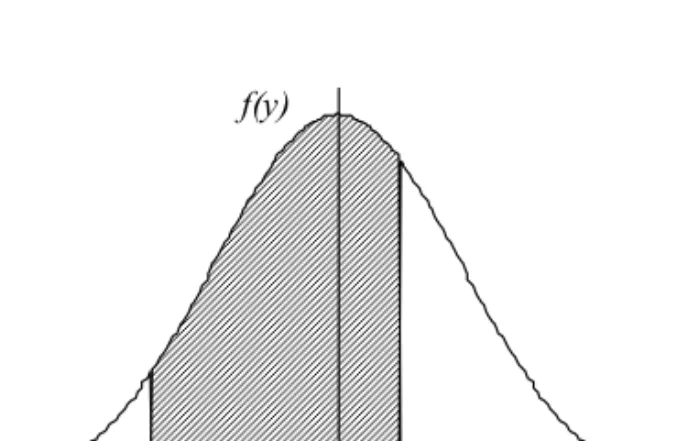
The Median of a sample of n observations y1,y2,...,yn is the value of the observation that is in the middle when observations are sorted from smallest to the largest. It is the value of the observation located such that one half of the area of a histogram is on the left and the other half is on the right. If n is an odd number the median is the value of the (n+1)/2-th observation. If n is an even number the median is the average of (n)/2-th and (n+2)/2-th observations.
The Mode of a sample of n observations y1,y2,...,yn is the value among the observations that has the highest frequency.
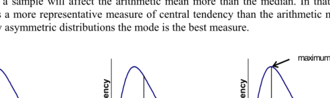
Figure 1.4 presents frequency distributions illustrating the mean, median and mode.
Although the mean is the measure that is most common, when distributions are asymmetric, the median and mode can give better information about the set of data. Unusually extreme values in a sample will affect the arithmetic mean more than the median. In that case the median is a more representative measure of central tendency than the arithmetic mean. For extremely asymmetric distributions the mode is the best measure.
frequency
mean (balance point)
frequency
median
50% 50% frequency
mode
maximum
Figure 1.4 Interpretation of mean, median and mode
1.4.3 Measures of Variability
Commonly used measures of variability are the range, variance, standard deviation and coefficient of variation.
Range is defined as the difference between the maximum and minimum values in a set of observations.
Sample variance (s2) of n observations (measurements) y1, y2,...,yn is:
1 )
( 2
2
−
=
∑
− ny
s i yi
This formula is valid if y is calculated from the same sample, i.e., the mean of a population is not known. If the mean of a population (µ) is known then the variance is:
n s2=
∑
i(yi−µ)2The variance is the average squared deviation about the mean.
The sum of squared deviations about the arithmetic mean is often called the corrected sum of squares or just sum of squares and it is denoted by SSyy. The corrected sum of squares can be calculated:
( )
n y y
y y
SS i i
i i
i i
yy
2 2
)2
(
∑ ∑
∑
− = −=
Further, the sample variance is often called the mean square denoted by MSyy, because:
1
2
= −
= n
MS SS
s yy yy
For grouped data, the sample variance with an unknown population mean is:
1 )
( 2
2
−
=
∑
− ny y s ifi i
where fi is the frequency of observation yi, and the total number of observations is n =
Σ
ifi. Sample standard deviation (s) is equal to square root of the variance. It is the average absolute deviation from the mean:s2
s=
Coefficient of variation (CV) is defined as:
% y100 CV = s
The coefficient of variation is a relative measure of variability expressed as a percentage. It is often easier to understand the importance of variability if it is expressed as a percentage.
This is especially true when variability is compared among sets of data that have different units. For example if CV for weight and height are 40% and 20%, respectively, we can conclude that weight is more variable than height.
1.4.4 Measures of the Shape of a Distribution
The measures of the shape of a distribution are the coefficients of skewness and kurtosis.
Skewness (sk) is a measure of asymmetry of a frequency distribution. It shows if deviations from the mean are larger on one side than the other side of the distribution. If the population mean (µ) is known, then skewness is:
(
−)(
−) ∑
− = i
i
s y n
sk n
3
2 1
1 µ
If the population mean is unknown, the sample mean (y) is substituted for µ and skewness is:
(
−)(
−) ∑
− = i
i
s y y n
n sk n
3
2 1
For a symmetric distribution skewness is equal to zero. It is positive when the right tail is longer, and negative when left tail is longer (Figure 1.5).
a) b)
Figure 1.5 Illustrations of skewness: a) negative, b) positive
Kurtosis (kt) is a measure of flatness or steepness of a distribution, or a measure of the heaviness of the tails of a distribution. If the population mean (µ) is known, kurtosis is:
1 4−3
−
=
∑
i is y
kt n µ
If the population mean is unknown, the sample mean (y) is used instead and kurtosis is:
( )
( )( )( ) ( )
(
2)(
3)
1 3 3
2 1
1 4 2
−
−
− −
−
−
−
−
= n nnn+ n
∑
y s y n n nkt i i
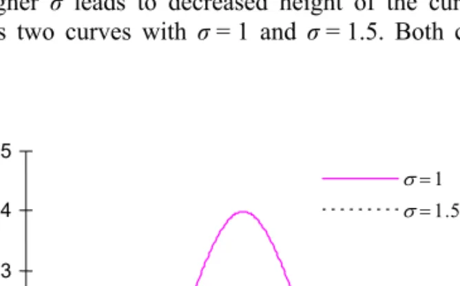
For variables such as weight, height or milk yield, frequency distributions are expected to be symmetric about the mean and bell-shaped. These are normal distributions. If observations follow a normal distribution then kurtosis is equal to zero. A distribution with positive kurtosis has a large frequency of observations close to the mean and thin tails. A distribution with a negative kurtosis has thicker tails and a lower frequency of observations close to the mean than does the normal distribution (Figure 1.6).
a) b)
Figure 1.6 Illustrations of kurtosis: a) positive, b) negative
1.4.5 Measures of Relative Position
Measures of relative position include percentiles and z-value.
The percentile value (p) of an observation yi, in a data set has 100p% of observations smaller than yi and has 100(1-p)% of observations greater than yi. A lower quartile is the 25th percentile, an upper quartile is 75th percentile, and the median is the 50th percentile.
The z-value is the deviation of an observation from the mean in standard deviation units:
s y zi yi−
=
Example: Calculate the arithmetic mean, variance, standard deviation, coefficient of variation, median and mode of the following weights of calves (kg):
260 260 230 280 290 280 260 270 260 300 280 290 260 250 270 320 320 250 320 220
Arithmetic mean:
n y=
∑
iyiΣ
i yi = 260 + 260 + … + 220 = 5470 kg 5. 20 273 5470=
=
y kg
Sample variance:
( )
1 1
) (
2 2 2
2
−
−
− =
= −
∑ ∑
∑
n n
y y
n y s y
i i
i i
i i
1510700 )
220 ...
260 260
( 2 2 2
2 = + + + =
∑
i iy kg2( )
3158 . 19 771
20 1510700 5470
2
2 − =
=
s kg2
Sample standard deviation:
77 . 27 3158 .
2 = 771 =
= s
s kg
Coefficient of variation:
% 15 . 10
% 273.5100 27.77
s100%= =
= y CV
To find the median the observations are sorted from smallest to the largest:
220 230 250 250 260 260 260 260 260 270 270 280 280 280 290 290 300 320 320 320
Since n = 20 is an even number, the median is the average of n/2 = 10th and (n+2)/2 = 11th observations when the data are sorted. The values of those observations are 270 and 270, respectively, and their average is 270, thus, the median is 270 kg. The mode is 260 kg because this is the observation with the highest frequency.
1.5 SAS Example
Descriptive statistics for the example set of weights of calves are calculated using SAS software. For a more detailed explanation how to use SAS, we recommend the exhaustive SAS literature, part of which is included in the list of literature at the end of this book. This SAS program consists of two parts: 1) the DATA step, which is used for entry and transformation of data, 2) and the PROC step, which defines the procedure(s) for data analysis. SAS has three basic windows: a Program window (PGM) in which the program is written, an Output window (OUT) in which the user can see the results, and LOG window in which the user can view details regarding program execution or error messages.
Returning to the example of weights of 20 calves:
SAS program:
DATA calves;
INPUT weight @@;
DATALINES;
260 260 230 280 290 280 260 270 260 300 280 290 260 250 270 320 320 250 320 220
;
PROC MEANS DATA = calves N MEAN MIN MAX VAR STD CV ; VAR weight;
RUN;
Explanation: The SAS statements will be written with capital letters to highlight them, although it is not generally mandatory, i.e. the program does not distinguish between small letters and capitals. Names that user assigns to variables, data files, etc., will be written with small letters. In this program the DATA statement defines the name of the file that contains data. Here, calves is the name of the file. The INPUT statement defines the name(s) of the variable, and the DATALINES statement indicates that data are on the following lines.
Here, the name of the variable is weight. SAS needs data in columns, for example, INPUT weight;
DATALINES;
260 260
… 220
;
reads values of the variable weight. Data can be written in rows if the symbols @@ are used with the INPUT statement. SAS reads observations one by one and stores them into a column named weight. The program uses the procedure (PROC) MEANS. The option DATA = calves defines the data file that will be used in the calculation of statistics, followed by the list of statistics to be calculated: N = the number of observations, MEAN = arithmetic mean, MIN = minimum, MAX = maximum, VAR = variance, STD= standard deviation, CV = coefficient of variation. The VAR statement defines the variable (weight) to be analyzed.
SAS output:
Analysis Variable: WEIGHT
N Mean Minimum Maximum Variance Std Dev CV --- 20 273.5 220 320 771.31579 27.77257 10.1545 ---
The SAS output lists the variable that was analyzed (Analysis variable: WEIGHT). The descriptive statistics are then listed.
Exercises
1.1. The number of eggs laid per month in a sample of 40 hens are shown below:
30 23 26 27 29 25 27 24 28 26 26 26 30 26 25 29 26 23 26 30 25 28 24 26 27 25 25 28 27 28 26 30 26 25 28 28 24 27 27 29 Calculate descriptive statistics and present a frequency distribution.
1.2. Calculate the sample variance given the following sums:
Σ
i yi = 600 (sum of observations);Σ
i yi2 = 12656 (sum of squared observations); n = 30 (number of observations)1.3. Draw the histogram of the values of a variable y and its frequencies f:
y 12 14 16 18 20 22 24 26 28
f 1 3 4 9 11 9 6 1 2
Calculate descriptive statistics for this sample.
1.4. The following are data of milk fat yield (kg) per month from 17 Holstein cows:
27 17 31 20 29 22 40 28 26 28 34 32 32 32 30 23 25
Calculate descriptive statistics. Show that if 3 kg are added to each observation, the mean will increase by three and the sample variance will stay the same. Show that if each observation is divided by two, the mean will be two times smaller and the sample variance will be four times smaller. How will the standard deviation be changed?
15
Chapter 2
Probability
The word probability is used to indicate the likelihood that some event will happen. For example, ‘there is high probability that it will rain tonight’. We can conclude this according to some signs, observations or measurements. If we can count or make a conclusion about the number of favorable events, we can express the probability of occurrence of an event by using a proportion or percentage of all events. Probability is important in drawing inferences about a population. Statistics deals with drawing inferences by using observations and measurements, and applying the rules of mathematical probability.
A probability can be a-priori or a-posteriori. An a-priori probability comes from a logical deduction on the basis of previous experiences. Our experience tells us that if it is cloudy, we can expect with high probability that it will rain. If an animal has particular symptoms, there is high probability that it has or will have a particular disease. An a- posteriori probability is established by using a planned experiment. For example, assume that changing a ration will increase milk yield of dairy cows. Only after an experiment was conducted in which numerical differences were measured, it can be concluded with some probability or uncertainty, that a positive response can be expected for other cows as well.
Generally, each process of collecting data is an experiment. For example, throwing a die and observing the number is an experiment.
Mathematically, probability is:
n P= m
where m is the number of favorable trials and n is the total number of trials.
An observation of an experiment that cannot be partitioned to simpler events is called an elementary event or simple event. For example, we throw a die once and observe the result.
This is a simple event. The set of all possible simple events is called the sample space. All the possible simple events in an experiment consisting of throwing a die are 1, 2, 3, 4, 5 and 6. The probability of a simple event is a probability that this specific event occurs. If we denote a simple event by Ei, such as throwing a 4, then P(Ei) is the probability of that event.
2.1 Rules about Probabilities of Simple Events
Let E1, E2,..., Ek be the set of all simple events in some sample space of simple events. Then we have:
1. The probability of any simple event occurring must be between 0 and 1 inclusively:
0 ≤ P(Ei) ≤ 1, i = 1,…, k
2. The sum of the probabilities of all simple events is equal to 1:
Σ
i P(Ei) =1Example: Assume an experiment consists of one throw of a die. Possible results are 1, 2, 3, 4, 5 and 6. Each of those possible results is a simple event. The probability of each of those events is 1/6, i.e., P(E1) = P(E2) = P(E3) = P(E4) = P(E5) = P(E6). This can be shown in a table:
Observation Event (Ei) P(Ei)
1 E1 P(E1) = 1/6
2 E2 P(E2) = 1/6
3 E3 P(E3) = 1/6
4 E4 P(E4) = 1/6
5 E5 P(E5) = 1/6
6 E6 P(E6) = 1/6
Both rules about probabilities are satisfied. The probability of each event is (1/6), which is less than one. Further, the sum of probabilities,
Σ
i P(Ei) is equal to one. In other words the probability is equal to one that any number between one and six will result from the throw of a die.Generally, any event A is a specific set of simple events, that is, an event consists of one or more simple events. The probability of an event A is equal to the sum of probabilities of the simple events in the event A. This probability is denoted with P(A). For example, assume the event that is defined as a number less than 3 in one throw of a die. The simple events are 1 and 2 each with the probability (1/6). The probability of A is then (1/3).
2.2 Counting Rules
Recall that probability is:
P = number of favorable trials / total number of trials
Or, if we are able to count the number of simple events in an event A and the total number of simple events:
P = number of favorable simple events / total number of simple events
A logical way of estimating or calculating probability is to count the number of favorable trials or simple events and divide by the total number of trials. However, practically this can often be very cumbersome, and we can use counting rules instead.
2.2.1 Multiplicative Rule
Consider k sets of elements of size n1, n2,..., nk. If one element is randomly chosen from each set, then the total number of different results is:
n1, n2, n3,..., nk
Example: Consider three pens with animals marked as listed:
Pen 1: 1,2,3 Pen 2: A,B,C Pen 3: x,y
The number of animals per pen are n1 = 3, n2 = 3, n3 = 2.
The possible triplets with one animal taken from each pen are:
1Ax, 1Ay, 1Bx, 1By, 1Cx, 1Cy 2Ax, 2Ay, 2Bx, 2By, 2Cx, 2Cy 3Ax, 3Ay, 3Bx, 3By, 3Cx, 3Cy
The number of possible triplets is: 3x3x2=18
2.2.2 Permutations
From a set of n elements, the number of ways those n elements can be rearranged, i.e., put in different orders, is the permutations of n elements:
Pn = n!
The symbol n! (factorial of n) denotes the product of all natural numbers from 1 to n:
n! = (1) (2) (3) ... (n) Also, by definition 0! = 1.
Example: In how many ways can three animals, x, y and z, be arranged in triplets?
n = 3
The number of permutations of 3 elements: P(3) = 3! = (1) (2) (3) = 6 The six possible triplets: xyz xzy yxz yzx zxy zyx
More generally, we can define permutations of n elements taken k at a time in particular order as:
( )
!!
, n k
Pnk n
= −
Example: In how many ways can three animals x, y and z be arranged in pairs such that the order in the pairs is important (xz is different than zx)?
(
3 2)
! 6! 3
, =
= −
k
Pn
The six possible pairs are: xy xz yx yz zx zy
2.2.3 Combinations
From a set of n elements, the number of ways those n elements can be taken k at a time regardless of order (xz is not different than zx) is:
( ) ( ) ( )
! 1 ...
1
!
!
!
k k n n n k n k
n k
n − − +
− =
=
Example: In how many ways can three animals, x, y, and z, be arranged in pairs when the order in the pairs is not important?
(
3 2)
! 3! 2
! 3 2
3 =
= −
=
k n
There are three possible pairs: xy xz yz
2.2.4 Partition Rule
From a set of n elements to be assigned to j groups of size n1, n2, n3,..., nj, the number of ways in which those elements can be assigned is:
!
!...
!
!
2
1 n nj
n n
where n = n1 + n2 + ... + nj
Example: In how many ways can a set of five animals be assigned to j=3 stalls with n1 = 2 animals in the first, n2 = 2 animals in the second and n3 = 1 animal in the third?
! 30 1 ! 2 ! 2
!
5 =
Note that the previous rule for combinations is a special case of partitioning a set of size n into two groups of size k and n-k.
2.2.5 Tree Diagram
The tree diagram illustrates counting, the representation of all possible outcomes of an experiment. This diagram can be used to present and check the probabilities of a particular
event. As an example, a tree diagram of possible triplets, one animal taken from each of three pens, is shown below:
Pen 1: 1, 2, 3 Pen 2: x, y Pen 3: A, B, C
The number of all possible triplets is:
(3)(3)(2) = 18 The tree diagram is:
Pen I 1 2 3 Pen II x y x y x y Pen III A B C A B C A B C A B C A B C A B C
The first triplet has animal 1 from Pen 1, animal x from pen 2, and animal A from Pen 3. If we assign the probabilities to each of the events then that tree diagram is called a probability tree.
2.3 Compound Events
A compound event is an event composed of two or more events. Consider two events A and B. The compound event such that both events A and B occur is called the intersection of the events, denoted by A ∩ B. The compound event such that either event A or event B occurs is called the union of events, denoted by A ∪ B. The probability of an intersection is P(A ∩ B) and the probability of union is P(A ∪ B). Also:
P(A ∪ B) = P(A) + P(B) - P(A ∩ B)
The complement of an event A is the event that A does not occur, and it is denoted by Ac. The probability of a complement is:
P(Ac) = 1 - P(A)
Example: Let the event A be such that the result of a throw of a die is an even number. Let the event B be such that the number is greater than 3.
The event A is the set: {2,4,6}
The event B is the set: {4,5,6}
The intersection A and B is an event such that the result is an even number and a number greater than 3 at the same time. This is the set:
(A ∩ B) = {4,6}
with the probability:
P(A ∩ B) =P(4) + P(6) = 2/6, because the probability of an event is the sum of probabilities of the simple events that make up the set.
The union of the events A and B is an event such that the result is an even number or a number greater than 3. This is the set:
(A ∪ B) = {2,4,5,6}
with the probability
P(A ∪ B) = P(2) + P(4) + P(5) + P(6) = 4/6
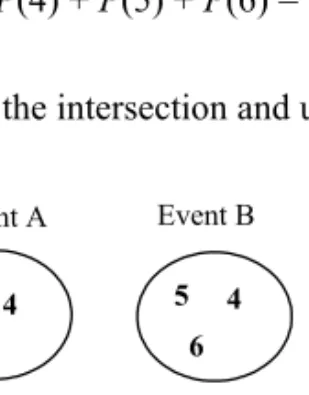
Figure 2.1 presents the intersection and union of the events A and B.
Event B Event A
6
2 4 5 4
6
2 4 5
6 A ∩ B
A ∪ B
Figure 2.1 Intersection and union of two events
A conditional probability is the probability that an event will occur if some assumptions are satisfied. In other words a conditional probability is a probability that an event B will occur if it is known that an event A has already occurred. The conditional probability of B given A is calculated by using the formula:
( )
) (
)
| (
A P
B A A P B
P = ∩
Events can be dependent or independent. If events A and B are independent then:
P(B | A) = P(B) and P(A | B) = P(B)
If independent the probability of B does not depend on the probability of A. Also, the probability that both events occur is equal to the product of each probability:
P(A ∩ B) = P(A) P(B)
If the two events are dependent, for example, the probability of the occurrence of event B depends on the occurrence of event A, then:
( )
) (
)
| (
A P
B A A P B
P ∩
=
and consequently the probability that both events occur is:
P(A ∩ B) = P(A) P(B|A)
An example of independent events: We throw a die two times. What is the probability of obtaining two sixes?
We mark the first throw as event A and the second as event B. We look for the probability P(A ∩ B). The probability of each event is: P(A) = 1/6, and P(B) = 1/6. The events are independent which means:
P(A ∩ B) = P(A) P(B) = (1/6) (1/6) = (1/36).
The probability that in two throws we get two sixes is (1/36).
An example of dependent events: From a deck of 52 playing cards we draw two cards. What is the probability that both cards drawn are aces?
The first draw is event A and the second is event B. Recall that in a deck there are four aces.
The probability that both are aces is P(A ∩ B). The events are obviously dependent, namely drawing of the second card depends on which card has been drawn first.
P(A = Ace) = (4/52) = (1/13).
P(B = Ace | A = Ace) = (3/51), that is, if the first card was an ace, only 51 cards were left and only 3 aces. Thus,
P(A ∩ B) = P(A) P(B|A) = (4/52) (3/51) = (1/221).
The probability of drawing two aces is (1/221).
Example: In a pen there are 10 calves: 2 black, 3 red and 5 spotted. They are let out one at the time in completely random order. The probabilities of the first calf being of a particular color are in the following table:
Ai P(Ai)
2 black A1 P(black) = 2/10
3 red A2 P(red) = 3/10
5 spotted A3 P(spotted) = 5/10
Here, the probability P(Ai) is the relative number of animals of a particular color. We can see that:
Σ
i P(Ai) = 1Find the following probabilities:
a) the first calf is spotted,
b) the first calf is either black or red,
c) the second calf is black if the first was spotted, d) the first calf is spotted and the second black,
e) the first two calves are spotted and black, regardless of order.
Solutions:
a) There is a total of 10 calves, and 5 are spotted. The