Last but not the least, I would like to express and deepest gratitude to my friends at IIT Hyderabad without whom this journey would have been very difficult if not impossible. In recent times, open source analysis software has been in demand to study various phenomena related to liquids and solids.
Introduction
Why the interest in droplet dynamics ?
Above all, with the introduction of newer fuel injection technologies such as CRDI (Common Rail Direct Injection), MPFI (Manifold Port Fuel Injection) and GDI (Gasoline Direct Injection) it becomes imperative to know everything there is to know. about droplet and bubble dynamics. Various attempts have been made over the years to explore the dynamics of droplets and bubbles and much still remains unknown.
Approach to investigation
- Analytical
- Experimental
- Numerical
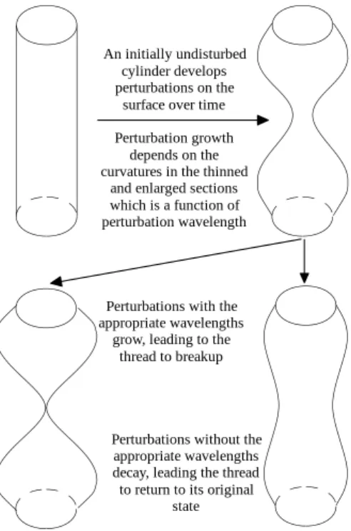
In other cases, the disturbance wavelength aids the pressure in the smaller area, leading to complete flushing of fluid out of the smaller area, eventually resulting in pinching. Using experiments, the flow can only be analyzed in those regions where there is sufficient concentration of the phase of interest.
Why OpenFOAM?
Apart from the provision to write a user-defined function, the user cannot touch the source code of the software. On the other hand, an open source code provides all kinds of freedom to the user to modify and modify and improvise on any domain he sees fit.
Scope of this thesis
Why SMAC (explicit) algorithm?
Therefore, very small time steps must be taken (∆t is of the order of 10−9) to correctly capture the physics of the flow. Also, since droplet breakup occurs, we need a very fine mesh to capture the baby drops.
The finite volume method
Typically, ∆xis is of the order of 10−7. A comparison of the order of temporal and spatial resolution concludes that the CFL number for the droplet breakup problem is well below 0.1.
The Governing Equations
Finite volume discretization
P stands for the current cell under consideration while all other cells labeled N,E,W,S (respectively north, east, west and south) are labeled relative to this cell. The basic assumption here is that the cell volume remains constant throughout the time step ∆t.
The SMAC algorithm
The solution to equation 2.20 gives the new pressure values which can then be substituted into equations and 2.19 to yield the final velocity field. For the next time step, the n+ 1 level values are transferred to the nth level and the algorithm is repeated. All the test cases performed and the reasons for performing them are mentioned below.
Navier Stokes Solving Skills: These tests assess how well the Navier Stokes equation is solved. The boundary condition nomenclature used below is derived from OpenFoam to facilitate replication and further use.
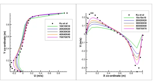
Testing the Navier Stoke’s equation solving capabilities of the solver
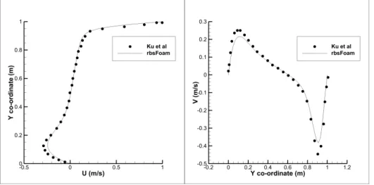
From the graphs above, it can be concluded that the results obtained from the simulations are consistent with those obtained from the experiments conducted by Ku et al. The satisfactory results for this test therefore show that the Navier Stokes solution algorithm implemented in rbsFoam is quite accurate. Second, it can be seen from Figures 3.3 and 3.2 that the peaks are not captured accurately enough.
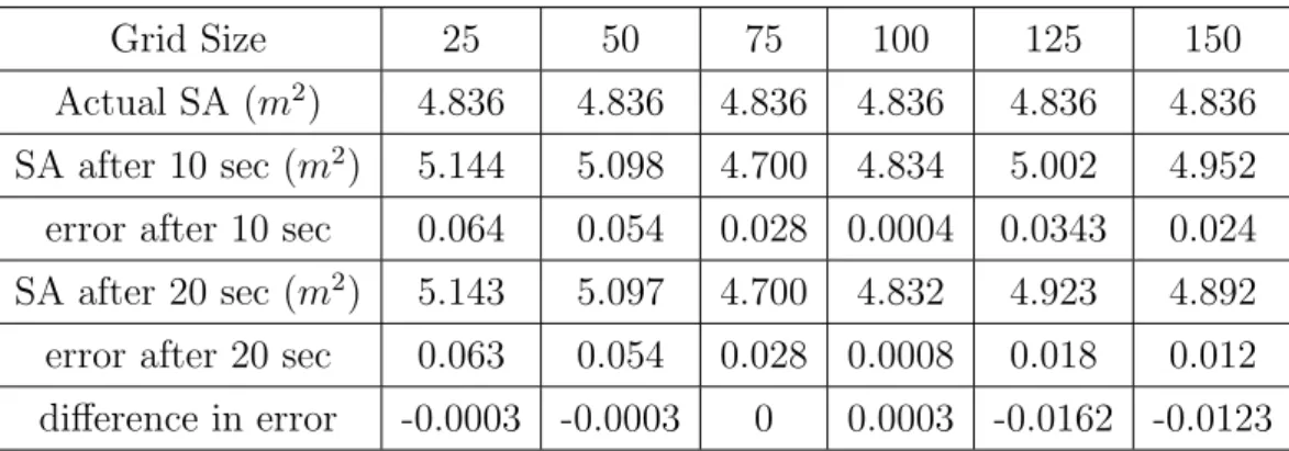
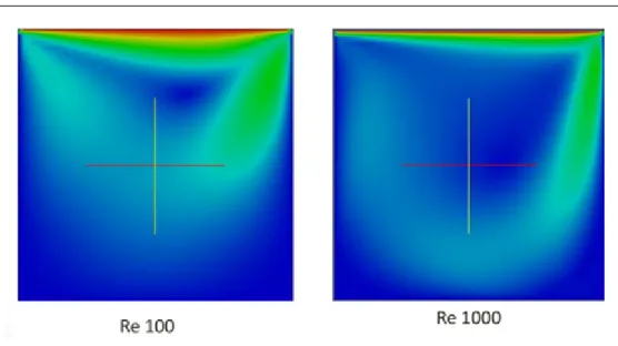
A mesh convergence study was also done to check what quality mesh would be good enough to best capture the phenomenon. The Re 1000 case was chosen for grid convergence study as it offers more unfavorable test conditions involving strong recirculation zones and eddies.
Testing the surface tension model implemen- tation of the solver
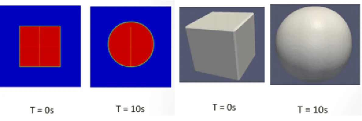
When solving any multiphase flow problem, surface tension appears as a source term in the Navier Stokes equation. Standard tests to verify the accuracy of the surface tension model include the quadratic or cubic bubble test (in 2D and 3D, respectively). When a steady state is reached, the circularity of the sphere is tested, which also serves as a measure of the accuracy of the surface tension model.
From the above equation it is clear that the calculation of the surface tension force depends on the calculation of the gradient, which in turn depends on the grid used. It can be clearly observed from the graph above that the behavior of the bubble when operated by the explicit algorithm is chaotic.
Static droplet test: a measure of Spurious currents
From the table it can be clearly seen that the magnitude of the L1 and L2 errors as well as the magnitude of the peak velocity in rbsFoam is large compared to the work of Menard et al.
Testing vof model
Note that here Nx and Ny stand for the number of cells along the x and y directions and not points. An important observation that can be made from the above table is that implicit as well as explicit solver have the same error, which is quite expected since neither solver actually solves for the velocity field. And yet we are able to achieve the same set of results in almost half the time compared to the implicit solver.
The error reported from rbsFoam is significantly large compared to the reference, indicating a poor implementation of the vof model. The results from Table 3.6 reveal that errors obtained from rbsFoam are slightly smaller compared to the standard reference code of Menard et al.
Testing NS, vof and ST modelling combined
- Droplet splashing
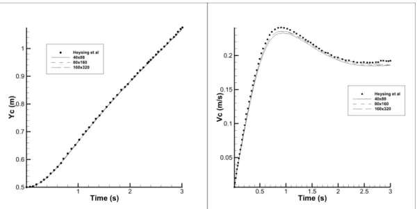
The important point to note here is that N stands for number of points different from 40x80 = 3200, as 40x80 or 80x160 indicates the number of cells along each direction. As can be clearly seen from plots in Figure 3.15, highly grid-convergent and accurate results are obtained for a density ratio of 10 an compared to that of Heysing et al. Again from Figures 3.15 and 3.16 it can be clearly seen that the simulation results obtained from rbsFoam are in good agreement with the experimental results obtained by Heysing et al.
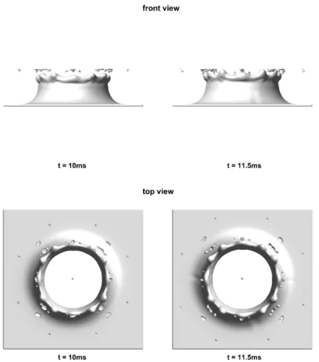
Therefore, it can be concluded from the above results that the solver is quite accurate and with the optimal case configuration obtained from the above test cases, a real-life problem can be successfully addressed. Although at first glance the results in Figure 3.19 may seem bad, the uncertainty in the estimation of the different diameters experimentally justifies the discrepancy.
Closure
For example, when a water droplet is subjected to an air blast, the water droplet has cohesive forces which manifest in the form of surface tension, trying to maintain the spherical shape of the droplet by holding it together. This inertial force experienced by the point usually depends on its size characterized by the diameter of the point D0. For example, when a drop is subjected to an air burst, for a We of 3.4 points it undergoes oscillatory deformation, but no separation is observed implying that the deforming inertial forces are weak compared to the surface tension force.
When Ne is further increased to a value of 100, the point undergoes sheet-thinning separation. In this dissolution mode, the droplet first deforms to form a thin sheet of liquid which then breaks up into smaller droplets.
Parameters affecting droplet collision
Case setup parameters
Results for different offset ratios and diam- eter ratio = 1.5
- Offset ratio x = 0
- Offset ratio x = 0.25
- Offset ratio x = 0.5
- Offset ratio x = 0.75
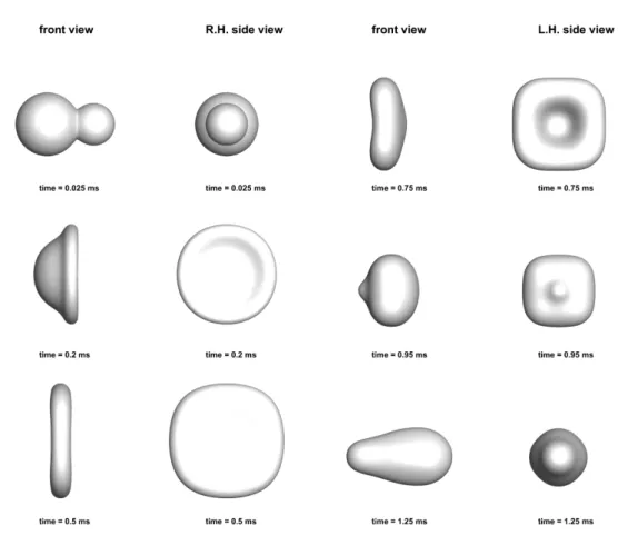
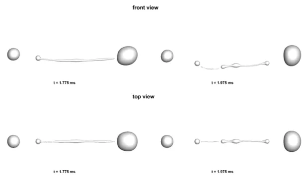
The smaller drop did not have enough energy to overcome the inertial and surface tension force of the larger drop and break away to the other side. Because the collision is now in the upper part of the larger droplet, a large lateral deformation occurs in this region. This region begins to move at slower speeds compared to the lower region of the droplet, causing elongation.
However, when the maximum lateral expansion is achieved at the expense of the kinetic energy of the smaller droplet, surface tension and viscous forces begin to pull the deformed lump of mass away. Because of this, most of the liquid appears to be divided into two spherical droplets.
Results for different diameter ratios and off- set ratio = 0.5
- Diameter ratio = 1
- Diameter Ratio = 1.25
- Diameter ratio = 1.75
For an offset ratio of 0.5, squeezing of a single child droplet was observed and finally for the largest offset ratio of 0.75, squeezing of both large droplets was observed, resulting in ligament separation that further broke off to yield child droplets. Because the ligament has insufficient surface area to retain the surface energy, it is further broken down into smaller droplets. Upon impact, the droplets merge and the resulting liquid mass begins to expand laterally.
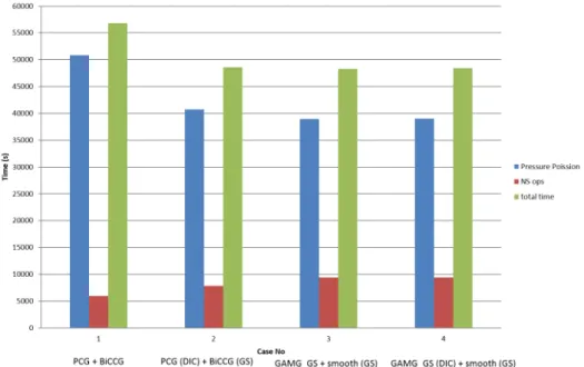
The ligament now has a larger surface area than the minimum required to hold this mass of fluid. Time required to solve the most computationally expensive Poisson pressure equation for various combinations of screeds, preconditioners, and screeds.
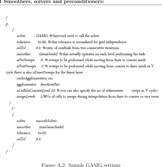
Smoothers, solvers and preconditioners
- Pre-conditioners
- Solvers
- Smoothers
Optimal choice of smoothers, preconditioners and solvers used to solve the U (velocity) and P (pressure) matrices. Below you will find a list of the preconditioners available in OpenFOAM, along with a brief explanation of their application. Note: The reciprocal of the diagonal is calculated and saved for reuse because multiplication is faster than division on most systems.
FDICPreconditioner - Faster version of the DICPreconditioner diagonal-based incomplete Cholesky preconditioner for symmetric matrices (symmetric equivalent of DILU) in which the reciprocal of the preconditioned diagonal and the upper coefficients divided by the diagonal are calculated and stored. Although the preconditioners discussed previously can significantly reduce the number of iterations, they normally do not reduce the mesh dependence of the number of iterations.
Multicore speedup analysis
Dynamic mesh refinement
The plots in Figure A.9 reveal that the results for any level of refinement are almost identical and roughly match the experimental results, suggesting that the base mesh of 40x80 cells was good enough to achieve the desired results. From the above plot in Figure A.11, it is clear that with dynamic mesh refinement there is a significant loss of accuracy. One way to avoid this is to initialize the volume fraction on a finer block as explained in Figure A.13 below.
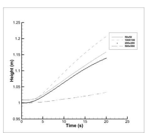
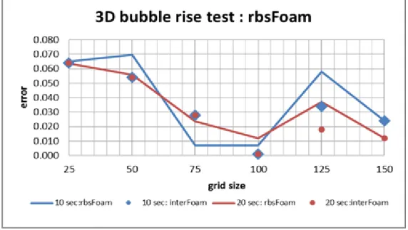
Again the bubble rise test case for a density ratio of 1000 is considered to numerically test the behavior of the bubble and compare the same with standard results. This is indicative of the fact that the source of error is interpolation from finer grid to coarser grid.