Constraint Propagation Analysis and Adjusted Systems

Constraint Propagation Analysis and Adjusted Systems

Gen Yoneda

Department of Mathematical Science, Waseda Univ., Japan yoneda@waseda.jp

Hisa-aki Shinkai

Computational Sci. Div., RIKEN (The Institute of Physical and Chemical Research), Japan hshinkai@riken.jp

Outline

• Constraint propagation analysis gives us an index of stability

• We try to unify previous treatments (such as hyperbolic and BSSN) by adjusting eqM.

Refs:

review article gr-qc/0209111 (Nova Science Publ.)

for Ashtekar form. PRD 60 (1999) 101502, CQG 17 (2000) 4799, CQG 18 (2001) 441 for ADM form. PRD 63 (2001) 124019, CQG 19 (2002) 1027

for BSSN form. PRD 66 (2002) 124003 general CQG 20 (2003) L31

This PDF is available at

www.f.waseda.jp/yoneda/mex.pdf

Plan of talks

1. Background of the problem

• ADM,BSSN

• hyperbolic

• asymptotically constrained 2. Constraint propagation analysis

• For time evolution systems with constraints in general

• Constraint Amplification Factors (CAF) as an index to express stability (partially new)

• examples (partially new) 3. adjusted systems

• For time evolution systems with constraints in general

• Example:Maxwell equations

• Example:Einstein eqautions(ADM) (partially new)

• Example:Einstein eqautions(BSSN) (partially new) 4. Numerical Demonstrations (new) → Hisaaki

5. Discussion (new) → Hisaaki

Best formulation of the Einstein eqs. for long-term stable & accurate simulation?

Many (too many) trials and errors, not yet a definit recipe.

time time

err or er ro r

Blow up

Blow up Blow up Blow up

ADM ADM

BSSN BSSN

Mathematically equivalent formulations, but differ in its stability!

strategy 0: Arnowitt-Deser-Misner formulation

strategy 1: Shibata-Nakamura’s (Baumgarte-Shapiro’s) modifications to the standard ADM strategy 2: Apply a formulation which reveals a hyperbolicity explicitly

strategy 3: Formulate a system which is “asymptotically constrained” against a violation of constraints

By adding constraints in RHS, we can kill error-growing modes

⇒ How can we understand the features systematically?

1 background of the problem

strategy 1 Shibata-Nakamura’s (Baumgarte-Shapiro’s) modifications to the standard ADM – define new variables (φ, γ ˜ _ij ,K, A ˜ _ij , Γ ˜ ⁱ ), instead of the ADM’s (γ _ij ,K _ij ) where

˜

γ _ij ≡ e ^{− 4φ} γ _ij , A ˜ _ij ≡ e ^{− 4φ} (K _ij − (1/3)γ _ij K), Γ ˜ ⁱ ≡ Γ ˜ ⁱ _jk γ ˜ ^jk , use momentum constraint in Γ ⁱ -eq., and impose det˜ γ _ij = 1 during the evolutions.

– The set of evolution equations become (∂ _t − L ^β )φ = − (1/6)αK,

(∂ _t − L ^β )˜ γ _ij = − 2α A ˜ _ij ,

(∂ _t − L ^β )K = α A ˜ _ij A ˜ ^ij + (1/3)αK ² − γ ^ij ( ∇ ⁱ ∇ ^j α),

(∂ _t − L ^β ) ˜ A _ij = − e ^{− 4φ} ( ∇ ⁱ ∇ ^j α) ^{T F} + e ^{− 4φ} αR ⁽³⁾ _ij − e ^{− 4φ} α(1/3)γ _ij R ⁽³⁾ + α(K A ˜ _ij − 2 ˜ A _ik A ˜ ^k _j )

∂ _t Γ ˜ ⁱ = − 2(∂ _j α) ˜ A ^ij − (4/3)α(∂ _j K )˜ γ ^ij + 12α A ˜ ^ji (∂ _j φ) − 2α A ˜ _k ^j (∂ _j γ ˜ ^ik ) − 2α Γ ˜ ^k _lj A ˜ ^j _k γ ˜ ^il

− ∂ _j β ^k ∂ _k γ ˜ ^ij − γ ˜ ^kj (∂ _k β ⁱ ) − γ ˜ ^ki (∂ _k β ^j ) + (2/3)˜ γ ^ij (∂ _k β ^k ) R _ij = ∂ _k Γ ^k _ij − ∂ _i Γ ^k _kj + Γ ^m _ij Γ ^k _mk − Γ ^m _kj Γ ^k _mi =: ˜ R _ij + R ^φ _ij

R ^φ _ij = − 2 ˜ D _i D ˜ _j φ − 2˜ g _ij D ˜ ^l D ˜ _l φ + 4( ˜ D _i φ)( ˜ D _j φ) − 4˜ g _ij ( ˜ D ^l φ)( ˜ D _l φ)

R ˜ _ij = − (1/2)˜ g ^lm ∂ _lm g ˜ _ij + ˜ g _k(i ∂ _{j )} Γ ˜ ^k + ˜ Γ ^k Γ ˜ _(ij)k + 2˜ g ^lm Γ ˜ ^k _l(i Γ ˜ _j)km + ˜ glm Γ ˜ ^k _im Γ ˜ _klj – No explicit explanations why this formulation works better.

AEI group (2000): the replacement by momentum constraint is essential.

strategy 2 Apply a formulation which reveals a hyperbolicity explicitly.

For a first order partial differential equations on a vector u,

∂ _t



 

 

 

u ₁ u ₂ ...



 

 

  =



 

 

  A



 

 

  ∂ _x



 

 

 

u ₁ u ₂ ...



 

 

 

characteristic part

+ B



 

 

 

u ₁ u ₂ ...



 

 

 

lower order part if the eigenvalues of A are

weakly hyperbolic all real.

strongly hyperbolic all real and ∃ a complete set of eigenvectors.

symmetric hyperbolic if A is real and symmetric (Hermitian).

Symmetric hyp.

Symmetric hyp.

Strongly hyp.

Strongly hyp.

Weakly hyp.

Weakly hyp.

Expectations

– Wellposed behaviour

symmetric hyperbolic system = ⇒ WELL-POSED , || u(t) || ≤ e ^κt || u(0) ||

– Better boundary treatments ⇐ = ∃ characteristic field.

– known numerical techniques in Newtonian hydrodynamics.

strategy2 Apply a formulation which reveals a hyperbolicity explicitly (cont.) Are hyperbolic formluations actulay helpful in numerical simulations?

Unfortunately, we do not have conclusive answer to it yet.

Theoretical issues

• Well-posedness of the non-linear hyperbolic formulations is obtained only locally in time domain.

• Energy inequality indicates boundedness of norm which does not forbid divergence

• The discussion of hyperbolcity only uses characteristic part of evolution equations, and ignore the non- characteristic part.

Numerical issues

• Earlier numerical comparisons reported the advantages of hyperbolic formulations, but they were against to the standard ADM formulation. [Cornell-Illinois, NCSA, ...]

• If the gauge functions are evolved with hyperbolic equations, then their finite propagation speeds may cause a pathological shock formation [Alcubierre].

• Some group [HS-GY, Hern] reported no drastic numerical differences between three hyperbolic levels, while other group [Calabresse] reported that strongly hyperbolic is good and weakly hyperbolic is bad. Of course, these statements only cast on a particular formulations and models to apply.

Proposed symmetric hyperbolic systems were not always the best one for numerics.

strategy 3 Formulate a system which is “asymptotically constrained” against a violation of constraints

“Asymptotically Constrained System”– Constraint Surface as an Attractor

t=0

Constrained Surface

(satisfies Einstein's constraints)

time time err or er ro r

Blow up Blow up

Stabilize?

Stabilize?

?

method 1: λ-system (Brodbeck et al, 2000)

– Add aritificial force to reduce the violation of con- straints

– To be guaranteed if we apply the idea to a sym- metric hyperbolic system.

method 2: Adjusted system (Yoneda HS, 2000, 2001) – We can control the violation of constraints by ad-

justing constraints to EoM.

– Eigenvalue analysis of constraint propagation equations may prodict the violation of error.

– This idea is applicable even if the system is not symmetric hyperbolic. ⇒

for the ADM/BSSN formulation, too!!

Idea of λ-system

Brodbeck, Frittelli, H¨ ubner and Reula, JMP40(99)909 We expect a system that is robust for controlling the violation of constraints

Recipe

1. Prepare a symmetric hyperbolic evolution system ^∂ t u = J ∂ _i u + K 2. Introduce λ as an indicator of violation of constraint

which obeys dissipative eqs. of motion

∂ _t λ = αC − βλ (α = 0, β > 0) 3. Take a set of (u, λ) as dynamical variables ∂ _t



 u λ







 A 0 F 0



 ∂ _i



 u λ





4. Modify evolution eqs so as to form

a symmetric hyperbolic system ^{∂ t}



 u λ



 =



 A F ¯ F 0



 ∂ _i



 u λ





Remarks

• BFHR used a sym. hyp. formulation by Frittelli-Reula [PRL76(96)4667]

• The version for the Ashtekar formulation by HS-Yoneda [PRD60(99)101502]

for controlling the constraints or reality conditions or both.

• Succeeded in evolution of GW in planar spacetime using Ashtekar vars. [CQG18(2001)441]

• Do the recovered solutions represent true evolution? by Siebel-H¨ ubner [PRD64(2001)024021]

80s 90s 2000s

A D M A D M

Shibata-Nakamura Shibata-Nakamura

95

Baumgarte-Shapiro Baumgarte-Shapiro

99

Nakamura-Oohara Nakamura-Oohara

87

Bona-Masso Bona-Masso

92

Anderson-York Anderson-York

99

ChoquetBruhat-York ChoquetBruhat-York

95-97

Frittelli-Reula Frittelli-Reula

96 62

Ashtekar Ashtekar

86

Yoneda-Shinkai Yoneda-Shinkai

00

Kidder-Scheel Kidder-Scheel -Teukolsky -Teukolsky

01

lambda-system lambda-system

99

adjusted-systema d j u s t e d - s y s t e m

01

Alcubierre Alcubierre

97

80s 90s 2000s

A D M A D M

Shibata-Nakamura Shibata-Nakamura

95

Baumgarte-Shapiro Baumgarte-Shapiro

99

Nakamura-Oohara Nakamura-Oohara

87

Bona-Masso Bona-Masso

92

Anderson-York Anderson-York

99

ChoquetBruhat-York ChoquetBruhat-York

95-97

Frittelli-Reula Frittelli-Reula

96 62

Ashtekar Ashtekar

86

Yoneda-Shinkai Yoneda-Shinkai

00

Kidder-Scheel Kidder-Scheel -Teukolsky -Teukolsky

01

NCSA

NCSA Potsdam Potsdam

G-code G-code H-code

H-code BSSN-code BSSN-code

Cornell-Illinois Cornell-Illinois

UWash UWash

Hern Hern

Caltech Caltech PennState

PennState

lambda-system lambda-system

99

adjusted-systema d j u s t e d - s y s t e m

01

Shinkai-Yoneda Shinkai-Yoneda Alcubierre

Alcubierre

97

Nakamura-Oohara

Nakamura-Oohara Shibata Shibata

80s 90s 2000s

A D M

Shibata-Nakamura

95

Baumgarte-Shapiro

99

Nakamura-Oohara

87

Bona-Masso

92

Anderson-York

99

ChoquetBruhat-York

95-97

Frittelli-Reula

96 62

Ashtekar

86

Yoneda-Shinkai

99

Kidder-Scheel -Teukolsky

01

NCSA AEI

G-code

H-code BSSN-code

Cornell-Illinois

UWash

Hern

Caltech PennState

lambda-system

99

ad ju st ed -s ys te m

01

Shinkai-Yoneda Alcubierre

97

Nakamura-Oohara Shibata

Iriondo-Leguizamon-Reula 97

LSU

Illinois

section 1 Background of the problem

section 2 Constraint propagation analysis

• For time evolution systems with constraints in general

• Constraint Amplification Factors (CAF) as an index to express stability (partially new)

• example1:Maxwell example2:ADM example3:BSSN

section 3 Adjusted systems

section 4 Numerical experiment

section 5 Discussion

For time evolution systems with constraints in general

∂ _t u ^a = f (u ^a , ∂u ^a , ∂∂u ^a ) evolution equations C ^α = C ^α (u ^a , ∂u ^a , ∂∂u ^a ) ≈ 0 constraints

If constraints are first class, constraint propagation takes this form

∂ _t C ^α = A ₀ C ^α + A ₁ ∂C ^α + A ₂ ∂∂C ^α + · · · constraint propagation

Analytically, constraints are satisfied during evolution. But numerically, does not.

By Fourier transformation, we rewrite constraint propagation with each modes, which is ODE.

∂ _t C ˆ ^α = A ₀ C ˆ ^α + A ₁ (i~k) ˆ C ^α + A ₂ (i~k)(i~k) ˆ C ^α + · · ·

= (A ₀ + A ₁ (i~k) + A ₂ (i~k)(i~k) + · · · )

| {z }

M

C ˆ ^α constraint propagation 2 constraint propagation matrix

we substitute background metric into M → M _bg

CAF := Eigenvalues M _bg Constraint Amplification Factors

By evaluating CAFs before simulations, we can predict constraint violation in

numerical evolution.

A Classification of Constraint Propagations

(C1) Asymptotically constrained :

Violation of constraints decays (converges to zero).

(C2) Asymptotically bounded :

Violation of constraints is bounded at a certain value.

(C3) Diverge :

At least one constraint will diverge.

Note that (C1) ⊂ (C2).

(C1) Decay (C2) Bounded

(C3) Diverge

time time

err or er ro r

Diverge Diverge

Constrained,

Constrained,

or Decay

or Decay

A Classification of Constraint Propagations (cont.)

∂ _t C = λC ⇒ C = C (0) exp(λt)

(C1) Asymptotically constrained : (Violation of constraints converges to zero.)

≈ all the real part of CAFs are negative

(C2) Asymptotically bounded : (Violation of constraints is bounded at a certain value.)

≈ all the real part of CAFs are non-positive

(C3) Diverge: (At least one constraint will diverge.)

≈ there exists CAF with positive real part

A Classification of Constraint Propagations (cont.)

∂ _t C = M C , CAF = Eigenvalues(M )

(C1) Asymptotically constrained : (Violation of constraints decays.)

⇔ all the real part of CAFs are negative

(C2) Asymptotically bounded : (Violation of constraints is bounded at a certain value.)

⇔ all the real part of CAFs are non-positive

and Jordan matrices for eigenvalues with zero real part are diagonal

⇐ all the real part CAFs are non-positive and M is diagonalizable (C3) Diverge: (At least one constraint will diverge.)

⇔ there exists CAF with positive real part

or there exists non diagonal Jordan matrix for eigenvalues with zero real part

A Classification of Constraint Propagations (cont.)

∂ _t C = M C , CAF = Eigenvalues(M )

(C1) Asymptotically constrained : (Violation of constraints decays.)

⇔ all the real part of CAFs are negative

(C2) Asymptotically bounded : (Violation of constraints is bounded at a certain value.)

⇔ all the real part of CAFs are non-positive

and Jordan matrices for eigenvalues with zero real part are diagonal

⇐ all the real part CAFs are non-positive and M is diagonalizable (C3) Diverge: (At least one constraint will diverge.)

⇔ there exists CAF with positive real part

or there exists non diagonal Jordan matrix for eigenvalues with zero real part

Each eigenvalue evaluation.

Real part: Nagative is better than zero and positive is worst.

Imaginary part: non-zero is better than zero for avoiding degeneracy.

A flowchart to classify the fate of constraint propagation.

Q1: Is there a CAF which real part is positive?

NO / YES

Q2: Are all the real parts of CAFs negative?

Q3: Is the constraint propagation matrix diagonalizable?

Q4: Is a real part of the degenerated CAFs is zero?

NO / YES

NO / YES

YES / NO

Diverge

Asymptotically Constrained

Asymptotically Bounded

Diverge

Asymptotically Bounded

Q5: Is the associated Jordan matrix diagonal?

NO / YES Asymptotically

Bounded

Example1: Maxwell equation

∂ _t E ⁱ = −c² ⁱ _j ^l ∂ _l B ^j , ∂ _t B ⁱ = c² ⁱ _j ^l ∂ _l E ^j C _E := ∂ _i E ⁱ ≈ 0, , C _B := ∂ _i B ⁱ ≈ 0,

∂ _t C _E = 0, ∂ _t C _B = 0

CAF = (0, 0) (asymptotically bounded) Example 2: ADM equation

∂ _t γ _ij = −2αK _ij + ∇ _i β _j + ∇ _j β _i ,

∂ _t K _ij = αR ⁽³⁾ _ij + αKK _ij − 2αK _ik K ^k _j − ∇ _i ∇ _j α + (∇ _i β ^k )K _kj + (∇ _j β ^k )K _ki + β ^k ∇ _k K _ij , H := R ⁽³⁾ + K ² − K _ij K ^ij ,

M _i := ∇ _j K ^j _i − ∇ _i K,

∂ _t H = β ^j (∂ _j H) − 2αγ ^ji (∂ _i M _j ) + 2αK H + α(∂ _l γ _mn )(2γ ^ml γ ^nj − γ ^mn γ ^lj )M _j − 4γ ^im (∂ _m α)M _i ,

∂ _t M _i = −(1/2)α(∂ _i H) + β ^j (∂ _j M _i ) + αK M _i − (∂ _i α)H − β ^k γ ^jm (∂ _i γ _mk )M _j + (∂ _i β _m )γ ^mj M _j . CAF = (0, 0, ± √

−k ² ) (in Minkowskii background) (asymptotically bounded)

Example 3: BSSN

∂ _t ^B ϕ = −(1/6)αK + (1/6)β ⁱ (∂ _i ϕ) + (∂ _i β ⁱ ),

∂ _t ^B γ ˜ _ij = −2α A ˜ _ij + ˜ γ _ik (∂ _j β ^k ) + ˜ γ _jk (∂ _i β ^k ) − (2/3)˜ γ _ij (∂ _k β ^k ) + β ^k (∂ _k γ ˜ _ij ),

∂ _t ^B K = −D ⁱ D _i α + α A ˜ _ij A ˜ ^ij + (1/3)αK ² + β ⁱ (∂ _i K ),

∂ _t ^B A ˜ _ij = −e ^−4ϕ (D _i D _j α) ^{T F} + e ^−4ϕ α(R _ij ^BSSN ) ^{T F} + αK A ˜ _ij − 2α A ˜ _ik A ˜ ^k _j + (∂ _i β ^k ) ˜ A _kj + (∂ _j β ^k ) ˜ A _ki

−(2/3)(∂ _k β ^k ) ˜ A _ij + β ^k (∂ _k A ˜ _ij ),

∂ _t ^B ˜Γ ⁱ = −2(∂ _j α) ˜ A ^ij + 2α(˜Γ ⁱ _jk A ˜ ^kj − (2/3)˜ γ ^ij (∂ _j K) + 6 ˜ A ^ij (∂ _j ϕ)) − ∂ _j (β ^k (∂ _k γ ˜ ^ij ) − γ ˜ ^kj (∂ _k β ⁱ )

− γ ˜ ^ki (∂ _k β ^j ) + (2/3)˜ γ ^ij (∂ _k β ^k )).

H ^BSSN = R ^BSSN + K ² − K _ij K ^ij , M ^BSSN _i = ∇ _j K ^j _i − ∇ _i K

G ⁱ = ˜Γ ⁱ − γ ˜ ^jk ˜Γ ⁱ _jk A = ˜ A _ij γ ˜ ^ij

S = ˜ γ − 1

constraint propagation is given in next page CAF = (0 (×3), ± √

−k ² (3 pairs)) (in Minkowskii background) (asymptotically bounded)

A Full set of BSSN constraint propagation eqs.

∂ _t ^BS



 

 

 

 

 

 

H ^BS M ⁱ

G ⁱ A S



 

 

 

 

 

 

=



 

 

 

 

 

 

A ₁₁ A ₁₂ A ₁₃ A ₁₄ A ₁₅

− (1/3)(∂ _i α) + (1/6)∂ _i αK A ₂₃ 0 A ₂₅

0 α˜ γ ^ij 0 A ₃₄ A ₃₅

0 0 0 β ^k (∂ _k S ) − 2α γ ˜

0 0 0 0 αK + β ^k ∂ _k



 

 

 

 

 

 



 

 

 

 

 

 

H ^BS M ^j

G ^j A S



 

 

 

 

 

 

A

₁₁

= +(2/3)αK + (2/3)α A + β

^k

∂

_k

A

₁₂

= − 4e

^−4ϕ

α(∂

_k

ϕ)˜ γ

^kj

− 2e

^−4ϕ

(∂

_k

α)˜ γ

^jk

A

₁₃

= − 2αe

^−4ϕ

A ˜

^k_j

∂

_k

− αe

^−4ϕ

(∂

_j

A ˜

_kl

)˜ γ

^kl

− e

^−4ϕ

(∂

_j

α) A − e

^−4ϕ

β

^k

∂

_k

∂

_j

− (1/2)e

^−4ϕ

β

^k

γ ˜

⁻¹

(∂

_j

S )∂

_k

+(1/6)e

^−4ϕ

˜ γ

⁻¹

(∂

_j

β

^k

)(∂

_k

S ) − (2/3)e

^−4ϕ

(∂

_k

β

^k

)∂

_j

A

₁₄

= 2αe

^−4ϕ

γ ˜

⁻¹

γ ˜

^lk

(∂

_l

ϕ) A ∂

_k

+ (1/2)αe

^−4ϕ

˜ γ

⁻¹

(∂

_l

A )˜ γ

^lk

∂

_k

+ (1/2)e

^−4ϕ

γ ˜

⁻¹

(∂

_l

α)˜ γ

^lk

A ∂

_k

+ (1/2)e

^−4ϕ

γ ˜

⁻¹

β

^m

γ ˜

^lk

∂

_m

∂

_l

∂

_k

− (5/4)e

^−4ϕ

γ ˜

⁻²

β

^m

γ ˜

^lk

(∂

_m

S )∂

_l

∂

_k

+ e

^−4ϕ

˜ γ

⁻¹

β

^m

(∂

_m

˜ γ

^lk

)∂

_l

∂

_k

+ (1/2)e

^−4ϕ

γ ˜

⁻¹

β

ⁱ

(∂

_j

∂

_i

γ ˜

^jk

)∂

_k

+(3/4)e

^−4ϕ

˜ γ

⁻³

β

ⁱ

˜ γ

^jk

(∂

_i

S )(∂

_j

S )∂

_k

− (3/4)e

^−4ϕ

˜ γ

⁻²

β

ⁱ

(∂

_i

˜ γ

^jk

)(∂

_j

S )∂

_k

+ (1/3)e

^−4ϕ

˜ γ

⁻¹

γ ˜

^pj

(∂

_j

β

^k

)∂

_p

∂

_k

− (5/12)e

^−4ϕ

˜ γ

⁻²

γ ˜

^jk

(∂

_k

β

ⁱ

)(∂

_i

S )∂

_j

+ (1/3)e

^−4ϕ

γ ˜

⁻¹

(∂

_k

γ ˜

^ij

)(∂

_j

β

^k

)∂

_i

− (1/6)e

^−4ϕ

γ ˜

⁻¹

˜ γ

^mk

(∂

_k

∂

_l

β

^l

)∂

_m

A

₁₅

= (4/9)αK A − (8/9)αK

²

+ (4/3)αe

^−4ϕ

(∂

_i

∂

_j

ϕ)˜ γ

^ij

+ (8/3)αe

^−4ϕ

(∂

_k

ϕ)(∂

_l

˜ γ

^lk

) + αe

^−4ϕ

(∂

_j

γ ˜

^jk

)∂

_k

+8αe

^−4ϕ

˜ γ

^jk

(∂

_j

ϕ)∂

_k

+ αe

^−4ϕ

˜ γ

^jk

∂

_j

∂

_k

+ 8e

^−4ϕ

(∂

_l

α)(∂

_k

ϕ)˜ γ

^lk

+ e

^−4ϕ

(∂

_l

α)(∂

_k

γ ˜

^lk

) + 2e

^−4ϕ

(∂

_l

α)˜ γ

^lk

∂

_k

+e

^−4ϕ

˜ γ

^lk

(∂

_l

∂

_k

α)

A

₂₃

= αe

^−4ϕ

γ ˜

^km

(∂

_k

ϕ)(∂

_j

γ ˜

_mi

) − (1/2)αe

^−4ϕ

Γ ˜

^m_kl

γ ˜

^kl

(∂

_j

γ ˜

_mi

)

+(1/2)αe

^−4ϕ

γ ˜

^mk

(∂

_k

∂

_j

˜ γ

_mi

) + (1/2)αe

^−4ϕ

γ ˜

⁻²

(∂

_i

S )(∂

_j

S ) − (1/4)αe

^−4ϕ

(∂

_i

γ ˜

_kl

)(∂

_j

γ ˜

^kl

) + αe

^−4ϕ

γ ˜

^km

(∂

_k

ϕ)˜ γ

_ji

∂

_m

+αe

^−4ϕ

(∂

_j

ϕ)∂

_i

− (1/2)αe

^−4ϕ

Γ ˜

^m_kl

γ ˜

^kl

˜ γ

_ji

∂

_m

+ αe

^−4ϕ

γ ˜

^mk

Γ ˜

_ijk

∂

_m

+ (1/2)αe

^−4ϕ

˜ γ

^lk

γ ˜

_ji

∂

_k

∂

_l

+(1/2)e

^−4ϕ

˜ γ

^mk

(∂

_j

γ ˜

_im

)(∂

_k

α) + (1/2)e

^−4ϕ

(∂

_j

α)∂

_i

+ (1/2)e

^−4ϕ

˜ γ

^mk

˜ γ

_ji

(∂

_k

α)∂

_m

A

₂₅

= − A ˜

^k_i

(∂

_k

α) + (1/9)(∂

_i

α)K + (4/9)α(∂

_i

K) + (1/9)αK∂

_i

− α A ˜

^k_i

∂

_k

A

₃₄

= − (1/2)β

^k

γ ˜

^il

γ ˜

⁻²

(∂

_l

S )∂

_k

− (1/2)(∂

_l

β

ⁱ

)˜ γ

^lk

γ ˜

⁻¹

∂

_k

+ (1/3)(∂

_l

β

^l

)˜ γ

^ik

γ ˜

⁻¹

∂

_k

− (1/2)β

^l

˜ γ

ⁱⁿ

(∂

_l

γ ˜

_mn

)˜ γ

^mk

γ ˜

⁻¹

∂

_k

+(1/2)β

^k

γ ˜

^il

γ ˜

⁻¹

∂

_l

∂

_k

A

₃₅

= − (∂

_k

α)˜ γ

^ik

+ 4α˜ γ

^ik

(∂

_k

ϕ) − α˜ γ

^ik

∂

_k

section 1 Background of the problem section 2 Constraint propagation analysis

section 3 Adjusted systems

• For time evolution systems with constraints in general

• Example:Maxwell equations

• Example:Einstein eqautions(Ashtekar)

• Example:Einstein eqautions(ADM) (partially new)

• Example:Einstein eqautions(BSSN) (partially new)

section 4 Numerical experiment

section 5 Discussion

Idea of adjusted system

Add constraint terms to evolution equations (adjust)

∂ _t u ^a = f (u ^a , ∂u ^a , ∂∂u ^a ) + F (C ^α , ∂C ^α , ∂∂C ^α )

constraint propagation changes depending on them, too

∂ _t C ^α = A ₀ C ^α + A ₁ ∂C ^α + A ₂ ∂∂C ^α + · · · + B ₀ C ^α + B ₁ ∂C ^α + B ₂ ∂∂C ^α + · · ·

CAF changes depending on them, too

We should adjust so that CAFs improve.

Advantage of adjusted system

1. Available even if the base system is not a symmetric hyperbolic.

2. Keep the number of the variables same with the original system.

3. Unified understanding for formulation problem is possible using the notions of

adjustment and CAF

Example: the Maxwell equations

Yoneda HS, CQG 18 (2001) 441 Maxwell evolution equations.

∂ _t E _i = c _i ^jk ∂ _j B _k + P _i C _E + Q _i C _B ,

∂ _t B _i = − c _i ^jk ∂ _j E _k + R _i C _E + S _i C _B ,

C _E = ∂ _i E ⁱ ≈ 0, C _B = ∂ _i B ⁱ ≈ 0,

 

 

 



 

 

 

sym. hyp ⇔ P _i = Q _i = R _i = S _i = 0, strongly hyp ⇔ (P _i − S _i ) ² + 4R _i Q _i > 0, weakly hyp ⇔ (P _i − S _i ) ² + 4R _i Q _i ≥ 0 Constraint propagation equations

∂ _t C _E = (∂ _i P ⁱ )C _E + P ⁱ (∂ _i C _E ) + (∂ _i Q ⁱ )C _B + Q ⁱ (∂ _i C _B ),

∂ _t C _B = (∂ _i R ⁱ )C _E + R ⁱ (∂ _i C _E ) + (∂ _i S ⁱ )C _B + S ⁱ (∂ _i C _B ),

 

 

 



 

 

 

sym. hyp ⇔ Q _i = R _i ,

strongly hyp ⇔ (P _i − S _i ) ² + 4R _i Q _i > 0, weakly hyp ⇔ (P _i − S _i ) ² + 4R _i Q _i ≥ 0 CAFs?

∂ _t



 C ˆ _E C ˆ _B



 =



 ∂ _i P ⁱ + P ⁱ k _i ∂ _i Q ⁱ + Q ⁱ k _i

∂ _i R ⁱ + R ⁱ k _i ∂ _i S ⁱ + S ⁱ k _i



 ∂ _l



 C ˆ _E C ˆ _B



 ≈



 P ⁱ k _i Q ⁱ k _i R ⁱ k _i S ⁱ k _i







 C ˆ _E C ˆ _B



 =: T



 C ˆ _E C ˆ _B





⇒ CAFs = (P ⁱ k _i + S ⁱ k _i ± (P ⁱ k _i + S ⁱ k _i ) ² + 4(Q ⁱ k _i R ^j k _j − P ⁱ k _i S ^j k _j ))/2 Therefore CAFs become negative-real when

P ⁱ k _i + S ⁱ k _i < 0, and Q ⁱ k _i R ^j k _j − P ⁱ k _i S ^j k _j < 0

Example: Maxwell adjusted (cont.)

GY HS, CQG 18 (2001) 441

∂ _t E ⁱ = −c² ⁱ _j ^l ∂ _l B ^j + κ∂ ⁱ C _E , ∂ _t B ⁱ = c² ⁱ _j ^l ∂ _l E ^j + κ∂ ⁱ C _B C _E := ∂ _i E ⁱ ≈ 0, , C _B := ∂ _i B ⁱ ≈ 0,

∂ _t C _E = κ∂ _i ∂ ⁱ C _E , ∂ _t C _B = κ∂ _i ∂ ⁱ C _B CAF = (−κ, −κ)

original Maxwell(κ = 0), CAF= (0, 0), averaged VN factor for FTCS=1.013

adjusted Maxwell(κ = 0.1), CAF= (−0.1, −0.1), averaged VN factor for FTCS=0.8017

adjusted Maxwell(κ = −0.1), CAF= (+0.1, +0.1), averaged VN factor for FTCS=1.2246 Adjustments also reduce the von Neumann factors.

In other words, adjustment is just like adding viscosity terms to evolution equations.

Example: the Ashtekar equations

HS Yoneda, CQG 17 (2000) 4799 Adjusted dynamical equations:

∂ _t E ˜ _a ⁱ = − i D ^j ( ^cb _a N _∼ E ˜ _c ^j E ˜ _b ⁱ ) + 2 D ^j (N ^[j E ˜ _a ^i] ) + i A ^b 0 _ab ^c E ˜ _c ⁱ +X _a ⁱ C ^H + Y _a ^ij C ^{M j} + P _a ^ib C ^Gb

adjust

∂ _t A ^a i = − i ^ab _c N _∼ E ˜ _b ^j F _ij ^c + N ^j F _ji ^a + D ⁱ A ^a 0 + ΛN _∼ E ˜ _i ^a +Q ^a _i C ^H + R _i ^aj C ^{M j} + Z _i ^ab C ^Gb

adjust

Adjusted and linearized:

X = Y = Z = 0, P _b ^ia = κ ₁ (iN ⁱ δ _b ^a ), Q ^a _i = κ ₂ (e ^{− 2} N _∼ E ˜ _i ^a ), R ^aj _i = κ ₃ ( − ie ^{− 2} N _∼ ^ac _d E ˜ _i ^d E ˜ _c ^j ) Fourier transform and extract 0th order of the characteristic matrix:

∂ _t



 

 



C ˆ ^H C ˆ ^{M i} C ˆ ^Ga



 

 

 =



 

 



0 i(1 + 2κ ₃ )k _j 0 i(1 − 2κ ₂ )k _i κ ₃ ^kj _i k _k 0 0 2κ ₃ δ _a ^j 0



 

 





 

 



C ˆ ^H C ˆ ^{M j}

C ˆ ^Gb



 

 



Eigenvalues:

0, 0, 0, ± κ ₃

− kx ² − ky ² − kz ² , ± ( − 1 + 2κ ₂ )(1 + 2κ ₃ )(kx ² + ky ² + kz ² )

In order to obtain non-positive real eigenvalues:

( − 1 + 2κ ₂ )(1 + 2κ ₃ ) < 0

3 Adjusted ADM systems

We adjust the standard ADM system using constraints as:

∂ _t γ _ij = − 2αK _ij + ∇ ⁱ β _j + ∇ ^j β _i , (1) +P _ij H + Q ^k _ij M ^k + p ^k _ij ( ∇ ^k H ) + q ^kl _ij ( ∇ ^k M ^l ), (2)

∂ _t K _ij = αR ⁽³⁾ _ij + αKK _ij − 2αK _ik K ^k _j − ∇ ⁱ ∇ ^j α + ( ∇ ⁱ β ^k )K _kj + ( ∇ ^j β ^k )K _ki + β ^k ∇ ^k K _ij , (3) +R _ij H + S ^k _ij M ^k + r ^k _ij ( ∇ ^k H ) + s ^kl _ij ( ∇ ^k M ^l ), (4) with constraint equations

H := R ⁽³⁾ + K ² − K _ij K ^ij , (5) M ⁱ := ∇ ^j K ^j _i − ∇ ⁱ K. (6)

We can write the adjusted constraint propagation equations as

∂ _t H = (original terms) + H ₁ ^mn [(2)] + H ₂ ^imn ∂ _i [(2)] + H ₃ ^ijmn ∂ _i ∂ _j [(2)] + H ₄ ^mn [(4)], (7)

∂ _t M ⁱ = (original terms) + M _1i ^mn [(2)] + M _2i ^jmn ∂ _j [(2)] + M _3i ^mn [(4)] + M _4i ^jmn ∂ _j [(4)]. (8)

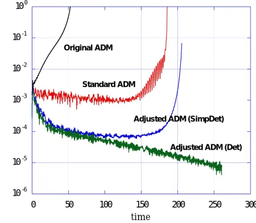
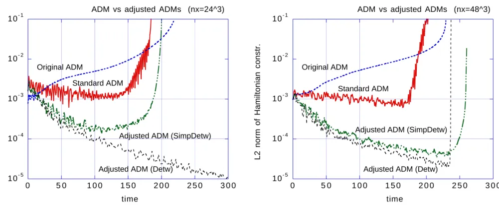
Standard ADM v.s. Original ADM in Minkowskii background

∂ _t γ _ij = −2αK _ij + ∇ _i β _j + ∇ _j β _i

∂ _t K _ij = αR ⁽³⁾ _ij + αKK _ij − 2αK _ik K ^k _j − ∇ _i ∇ _j α + (∇ _i β ^k )K _kj + (∇ _j β ^k )K _ki +β ^k ∇ _k K _ij + κ _F αγ _ij H

standard : κ _F = 0, original : κ _F = −1/4 CAFs = (0, 0, ± ^r −k ² (1 + 4κ _F ))

standard : (0, 0, =, =) (asymptotically bounded) original : (0, 0, 0, 0) (diverge)

Standard ADM is better than original ADM.

Example 1: standard ADM vs original ADM (in Schwarzschild coordinate)

- 1 -0.5 0 0.5 1

0 5 1 0 1 5 2 0

no adjustments (standard ADM)

Real / Imaginary parts of Eigenvalues (AF)

rsch

( a )

-0.5 0 0.5

0 5 1 0 1 5 2 0

original ADM (κ

F= - 1/4)

rsch

( b )

Real / Imaginary parts of Eigenvalues (AF)

Figure 1: Amplification factors (AFs, eigenvalues of homogenized constraint propagation equations) are shown for the standard Schwarzschild coordinate, with (a) no adjustments, i.e., standard ADM, (b) original ADM (κ

_F

= − 1/4). The solid lines and the dotted lines with circles are real parts and imaginary parts, respectively. They are four lines each, but actually the two eigenvalues are zero for all cases. Plotting range is 2 < r ≤ 20 using Schwarzschild radial coordinate. We set k = 1, l = 2, and m = 2 throughout the article.

∂ _t γ _ij = − 2αK _ij + ∇ ⁱ β _j + ∇ ^j β _i ,

∂ _t K _ij = αR ⁽³⁾ _ij + αKK _ij − 2αK _ik K ^k _j − ∇ ⁱ ∇ ^j α + ( ∇ ⁱ β ^k )K _kj + ( ∇ ^j β ^k )K _ki + β ^k ∇ ^k K _ij + κ _F αγ _ij H ,

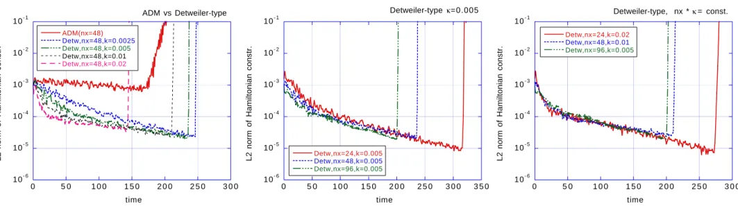
Example 2: Detweiler-type adjusted (in Schwarzschild coord.)

- 1 -0.5 0 0.5 1

0 5 1 0 1 5 2 0

Detweiler type, κ

L = + 1/2 ( b )

Real / Imaginary parts of Eigenvalues (AF)

rsch

- 1 -0.5 0 0.5 1

0 5 1 0 1 5 2 0

Detweiler type, κ

L = - 1/2

Real / Imaginary parts of Eigenvalues (AF)

( c )

rsch

Figure 2: Amplification factors of the standard Schwarzschild coordinate, with Detweiler type adjustments. Multipliers used in the plot are (b) κ

_L

= +1/2, and (c) κ

_L

= − 1/2.

∂ _t γ _ij = (original terms) + P _ij H ,

∂ _t K _ij = (original terms) + R _ij H + S ^k _ij M ^k + s ^kl _ij ( ∇ ^k M ^l ),

where P _ij = − κ _L α ³ γ _ij , R _ij = κ _L α ³ (K _ij − (1/3)Kγ _ij ),

S ^k _ij = κ _L α ² [3(∂ _(i α)δ _j) ^k − (∂ _l α)γ _ij γ ^kl ], s ^kl _ij = κ _L α ³ [δ _(i ^k δ _j) ^l − (1/3)γ _ij γ ^kl ],

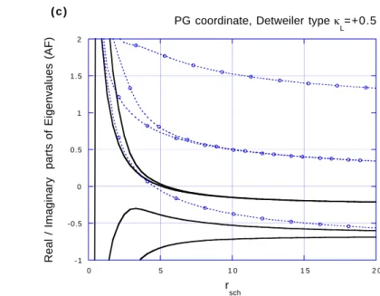
Example 4: Detweiler-type adjusted (in iEF/PG coord.)

- 1 -0.5 0 0.5 1 1.5 2

0 5 1 0 1 5 2 0

iEF coordinate, Detweiler type κ

L=+0.5 ( b )

Real / Imaginary parts of Eigenvalues (AF)

rsch

- 1 -0.5 0 0.5 1 1.5 2

0 5 1 0 1 5 2 0

PG coordinate, Detweiler type κ

L=+0.5 ( c )

Real / Imaginary parts of Eigenvalues (AF)

rsch

Figure 4: Similar comparison for Detweiler adjustments. κ

_L

= +1/2 for all plots.