저작자표시-비영리-변경금지 2.0 대한민국 이용자는 아래의 조건을 따르는 경우에 한하여 자유롭게
l 이 저작물을 복제, 배포, 전송, 전시, 공연 및 방송할 수 있습니다. 다음과 같은 조건을 따라야 합니다:
l 귀하는, 이 저작물의 재이용이나 배포의 경우, 이 저작물에 적용된 이용허락조건 을 명확하게 나타내어야 합니다.
l 저작권자로부터 별도의 허가를 받으면 이러한 조건들은 적용되지 않습니다.
저작권법에 따른 이용자의 권리는 위의 내용에 의하여 영향을 받지 않습니다. 이것은 이용허락규약(Legal Code)을 이해하기 쉽게 요약한 것입니다.
Disclaimer
저작자표시. 귀하는 원저작자를 표시하여야 합니다.
비영리. 귀하는 이 저작물을 영리 목적으로 이용할 수 없습니다.
변경금지. 귀하는 이 저작물을 개작, 변형 또는 가공할 수 없습니다.
Master's Thesis
Nam Kyu Kim
Department of Urban and Environmental Engineering (Environmental Science and Engineering)
Ulsan National Institute of Science and Technology
2023
Investigation on seasonal and spatial variation, source identification, and risk assessment of parent,
nitrated, and oxygenated PAHs using passive air
samplers in Ulsan, Korea
Nam Kyu Kim
Department of Urban and Environmental Engineering (Environmental Science and Engineering)
Ulsan National Institute of Science and Technology
Investigation on seasonal and spatial variation, source identification, and risk assessment of parent,
nitrated, and oxygenated PAHs using passive air
samplers in Ulsan, Korea
I
Abstract
Polycyclic aromatic hydrocarbons (PAHs) are ubiquitous toxic air pollutants, which are mainly emitted through incomplete combustion together with derivates PAHs such as OPAHs and NPAHs.
Additionally, NOPAHs are also formed through secondary formation by a reaction between existing PAHs and atmospheric oxidants such as nitrate, ozone, and OH radicals. In this study, the level of concentration, seasonal and spatial variation, source-receptor relationship, and potential cancer risk of 21 PAHs, 9 OPAHs, and 17 NPAHs was investigated using passive air samplers (PASs) in Ulsan.
The air samples were pretreated through Soxhlet extraction, clean-up using silica gel column for PAHs and silica/alumina gel column for NOPAHs, and concentration. After that, PAHs were analyzed using a gas chromatography/mass spectrometry-electron ionization (GC/MS-EI) meanwhile NOPAHs were analyzed using a gas chromatography/mass spectrometry-negative chemical ionization (GC/MS- NCI). The abundant compounds consisted of low and middle-molecular weight compounds (2-, 3-, and 4-rings). The level of concentration is similar compared to other studies. Through the spatial distribution, it was confirmed that each target compound had other emission sources by season. PAHs are mainly emitted by petrochemical industrial and non-ferrous metal industrial complexes in the warm season and by the automobile industrial complex in the cold season. OPAHs were mainly emitted near the automobile industrial complex during all seasons. On the other hand, it was difficult to find clear emission sources for NPAHs.
To identify the relationship between emission source and receptor, correlation analysis and diagnostic were performed. As a result of correlation analysis between PAHs and derivative PAHs, there are significant positive correlations suggesting they were emitted from similar emission sources. The emission sources and formation pathways of target compounds were investigated using the diagnostic ratio. PAHs were mainly affected by liquid fossil fuel combustion during total sampling period, greatly influenced by petroleum evaporation in warm seasons, and clearly influenced by biomass burning and coal combustion in cold seasons. For NPAHs, it was generated through secondary generation by OH radicals.
Potential cancer risk was assessed by using the incremental lifetime cancer risk (ILCR) model. In advance, BaPeq was calculated using individual concentrations (Ci) and toxic equivalent factors (TEFi).
Through the spatial distribution of risk, PAHs were higher in industrial complexes and NPAHs in non- ferrous metal industrial complexes. It is the first study to investigate source identification and health risk assessment for PAHs, NPAHs, and OPAHs using PUF-PAS in Korea.
II
Contents
Abstract ... I Contents ... II List of Figures ... III
List of Tables ... V
Ⅰ. Introduction ... 1
Ⅱ. Material and Methods ... 8
2.1. Chemicals and material ... 8
2.2 Passive air sampling ... 9
2.3 Analysis procedure and instrumental condition ... 10
2.4 Quality assurance and Quality controls (QA/QC) ... 11
2.5 Calculation of PAHs concentration in air ... 13
2.6. Meteorological and criteria/hazardous air pollutant data ... 14
2.7 Statistical tools ... 14
2.8 Risk assessments ... 14
Ⅲ. Results and Discussion ... 16
3.1. Calculation of sampling rates ... 16
3.2. Level of concentration of target compounds ... 17
3.3. Spatial distribution ... 21
3.4. Source identification ... 24
3.4.1 Correlation analysis... 24
3.4.1 Diagnostic ratio ... 24
3.5 Risk assessment ... 30
Ⅳ. Conclusion ... 33
Reference ... 35
Supplementary information ... 42
Acknowledgement ... 50
III
List of Figures
Figure 1. The number literature of studies on NPAHs and OPAHs yearly. ... 2
Figure 2. Chemical structures and name of the investigated target compounds of (a) PAHs, (b) NPAHs, and (c) OPAHs. ... 4
Figure 3. Air samplers for air pollutant monitoring. ... 6
Figure 4. Industrial areas and wind direction as seasonal in Ulsan. ... 7
Figure 5. The sampling sites and industrial areas in this study area. ... 9
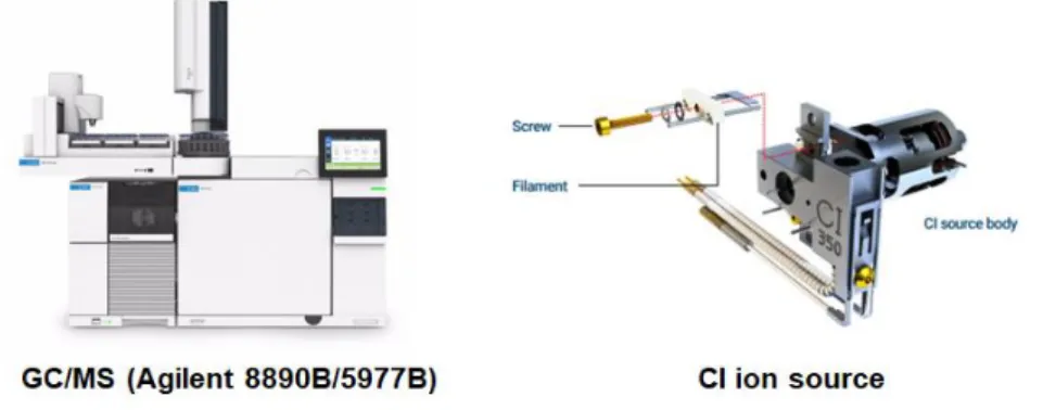
Figure 6. Gas chromatography/mass spectrometry-negative chemical ionization (GC/MS-NCI) ... 10
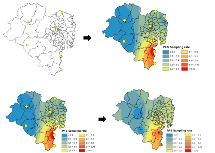
Figure 7. The method of calculation on average sampling rate. ... 16
Figure 8. The level of PAHs, OPAHs, and NPAHs in this study. ... 18
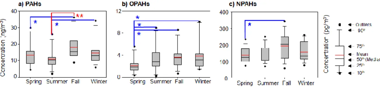
Figure 9. Boxplot of seasonal concentrations of a) PAHs, b) OPAHs, and c) NPAHs... 18
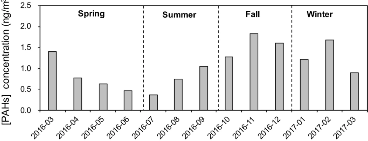
Figure 10. Average concentration of PAHs monthly at hazardous air pollutant stations. ... 19
Figure 11. Average monthly temperature and humidity at ASOS station... 19
Figure 12. Seasonal fraction and concentration of PAHs, OPAHs, and NPAHs. ... 20
Figure 13. Spatial distribution of PAHs in Ulsan, in (a) spring, (b) summer, (c) fall, and (d) winter. . 22
Figure 14. Spatial distribution of OPAHs in Ulsan, in (a) spring, (b) summer, (c) fall, and (d) winter. ... 22
Figure 15. Spatial distribution of NPAHs in Ulsan, in (a) spring, (b) summer, (c) fall, and (d) winter. ... 23
Figure 16. Wind field in Ulsan, in (a) spring, (b) summer, (c) fall, and (d) winter. ... 23
Figure 17. Ratio of 9-Fluorenone/Fluorene at each sampling site ... 26
Figure 18. Ratio of 7,12-Benz[a]anthracenedione /Benzo[a]anthracene at each sampling site. ... 26
Figure 19. Ratio of 9,10-Anthracenedione/Anthracene at each sampling site ... 26
Figure 20. Scatter plot of two diagnostic ratios of Flt/Flt+Pyr and Flu/Flu+Pyr. ... 27
Figure 21. Two-scatter plots of two diagnostic ratios of Flu/Flu+Pyr and IcdP/IcdP+BghiP by season and land-use. ... 28
IV
Figure 22. Diagnostic ratio of 1-NNap/2-NNap. ... 29
Figure 23. Diagnostic ratio of 2+3-NFlt/2-NPyr. ... 29
Figure 24. Diagnostic ratio of 2+3-NFlt/1-NPyr. ... 29
Figure 25. (a) Fraction and (b) Toxic equivalent concentration (TEQ) by seasonal. ... 30
Figure 26. Stack bar of the total incremental lifetime cancer risk (ILCR) of PAHs and NPAHs... 30
Figure 27. Spatial distribution of the total incremental lifetime cancer risk (ILCR) for PAHs. ... 32
Figure 28. Spatial distribution of the total incremental lifetime cancer risk (ILCR) for NPAHs... 32
Figure S1. Chromatograms of calibration standard and real sample. ... 42
Figure S2. Spatial distribution of NO2 in Ulsan, in (a) spring, (b) summer, (c) fall, and (d) winter. ... 48
Figure S3. Spatial distribution of population density (people/km2) in Ulsan. ... 48
V
List of Tables
Table 1. IARC Classification for PAH and NPAHs. ... 5
Table 2. Recovery rate of surrogates ... 11
Table 3. MDL and IDL for target compounds. ... 12
Table 4. Toxic equivalent factors of PAHs and NPAHs ... 15
Table 5. Result of correlation analysis between NPAHs and CAPs. ... 25
Table 6. Result of correlation analysis between OPAHs and CAPs ... 25
Table S1. List of physicochemical properties of target compounds consisting of chemical names, abbreviations, CAS number, MW: molecular weight, H: Henry’s law constant, boiling point, melting point, KOA: octanol-air partition coefficient, U: Internal energy. ... 42,43 Table S2. Comparison of total mean concentration of PAHs (ng/m3), OPAHs (ng/m3), and NPAHs (pg/m3) in other studies. ... 44
Table S3. Result of correlation analysis between NOPAHs and CAPs at spring. ... 45
Table S4. Result of correlation analysis between NOPAHs and CAPs at summer... 45
Table S5. Result of correlation analysis between NOPAHs and CAPs at fall. ... 46
Table S6. Result of correlation analysis between NOPAHs and CAPs at winter. ... 46
Table S7. Result of correlation analysis between PAHs and OPAHs. ... 48
Table S8. Result of correlation analysis between PAHs and NPAHs ... 48
Table S9. Result of correlation analysis between NPAHs and OPAHs. ... 48
1
Ⅰ. Introduction
Polycyclic aromatic hydrocarbons (PAHs) are having two or more aromatic benzene rings and are ubiquitous organic contaminants, which are known for having multimedia fate. They have carcinogenic and/or mutagenic properties(IARC, 2004, 2010), thus among them, sixteen PAHs have been classified by the United States Environmental Protection Agency (US-EPA) as priority pollutants(Choi, 2014; Thang et al., 2020). In the atmosphere, PAHs with low molecular weights having 2- or 3- rings exist in the gaseous phase, whereas high molecular weights having 4-, 5-, and 6- rings exist in association with airborne particulates(Masih et al., 2012; Singh et al., 2021). PAHs are mainly emitted into the atmosphere from incomplete combustion such as industrial activities, vehicular exhausts, and biomass burning (ChooChuay et al., 2020; Tsai et al., 2004). Emitted PAHs can be reacted with atmospheric oxidants such as NO3-, O3, and OH radicals(Arey et al., 1986;
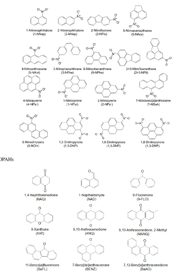
Kojima et al., 2010; Pitts Jr et al., 1978; J. Zhang et al., 2018a), consequently producing derivate PAHs, which are nitrated PAHs (NPAHs) or oxygenated PAHs (OPAHs). They contain at least one nitro-functional group and a carboxyl group or ketone group on the parent PAH (pPAHs). The investigated target compounds of PAHs, NPAHs, and OPAHs are arranged in Figure 2. They are also emitted from primary sources like the incomplete combustion of diesel(Leotz-Gartziandia et al., 2000;
Li et al., 2018). Some NOPAHs are more toxic than pPAHs due to directly acting mutagenic and carcinogenic properties(Pedersen et al., 2005; Wang et al., 2011). The International Agency for Research on Cancer (IARC) has classified benzo[a]pyrene (BaP) under Group 1 as carcinogenic to humans, BaA and Chr under Group 2A as probable carcinogens to humans, as well as 1-Nitropyrne (1-NPyr) and 6-nitrochrysene (6-NChr) in Group 2A(IARC, 2012). Several PAHs and NPAHs are considered possibly carcinogenic to humans in Group B(IARC, 2014)(Table 1).
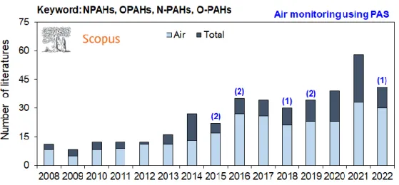
PAHs studies have been conducted worldwide. In recent years, studies considering not only PAHs but also derivatives PAHs such as NPAHs and OPAHs are increasing (Figure 1). Research on analytical methods for NOPAHs has been underway, several papers reported that gas chromatography/mass spectrometry-negative chemical ionization (GC/MS-NCI) has higher sensitivity for NOPAHs than gas chromatography/mass spectrometry-electron ionization (GC/MS-EI)(Albinet et al., 2006; Galmiche et al., 2021). Generally, the air concentration of NOPAHs is one or two orders of magnitude lower than pPAHs (Albinet et al., 2008; Liu et al., 2017). The several papers reported NOPAHs have a lower emission factor about 10~1000 times than pPAHs(Percy & Foster, 2011; Shen et al., 2013; Shen et al., 2012; Vicente et al., 2015; Zhao et al., 2020); Thus, high sensitivity is essential to investigate NOPAHs with low atmospheric concentrations. Since the late 2000s, atmospheric monitoring of NOPAHs has been significantly conducted to investigate the atmospheric behavior such as air concentration, emission sources, secondary formation, and gas-particulate partitioning(Albinet et al.,
2
2007; Ringuet, Leoz-Garziandia, et al., 2012; Tomaz et al., 2016). In Korea, there are several papers on NOPAHs(Lee et al., 2018; Lee et al., 2013; Park et al., 2010; Shin et al., 2022). These papers are focused on OPAHs, and no air concentrations have been reported for NPAHs. Although many studies have been conducted on NOPAHs, most of the studies focused on NOPAHs bound in the particulate phase(Huang et al., 2014; Kalisa et al., 2019; Lixin et al., 2020; J. Zhang et al., 2018b). There were few papers using passive air sampler. Therefore, in order to investigate high-resolution spatial distribution and the relationship between source and receptor, it is necessary to conduct air monitoring on NOPAHs using passive air samplers in Korea.
Figure 1. The number literature of studies on NPAHs and OPAHs yearly.
3 (a) PAHs
4 (b) NPAHs
(c) OPAHs
Figure 2. Chemical structures and name of the investigated target compounds of (a) PAHs, (b) NPAHs, and (c) OPAHs.
5 Table 1. IARC Classification for PAH and NPAHs.
PAHs Abbreviation IARC Classification
Fluorene Flu 3
Phenanthrene Phe 3
Anthracene Ant 3
Fluoranthene Flt 3
Pyrene Pyr 3
Benzo[c]phenanthrene BcP 2B
Benz[a]anthracene BaA 2B
Chrysene Chr 2B
Benzo[b]fluoranthene BbF 2B
Benzo[j]fluoranthene BjF 2B
Benzo[k]fluoranthene BkF 2B
7,12-Dimethylbenz[a]anthracene DMBA -
Benzo[e]pyrene BeP 3
Benzo[a]pyrene BaP 1
3-Methylcholanthrene 3MCA -
Indeno[1,2,3-cd]pyrene IcdP 2B
Dibenz[a,h]anthracene DahA 2A
Benzo[g,h,i]perylene BghiP 3
Dibenzo[a,i]pyrene DbaiP 2B
Dibenzo[a,h]pyrene DbahP 2B
Dibenzo[a,l]pyrene DbalP 2A
NPAHs Abbreviation IARC Classification
2-Nitrofluorene 2-NFlu 2B
1-Nitropyrene 1-NPyr 2A
2-Nitropyrene 2-NPyr 2B
4-Nitropyrene 4-NPyr 2B
6-Nitrochyrsene 6-NChr 2A
1.3-Dinitropyrene 1,3-DNP 2B
1,8-Dinitropyrene 1,8-DNP 2B
1,6-Dinitropyrene 1,6-DNP 2B
6
For monitoring atmospheric PAHs, active air samplers (AASs) or passive air samplers (PASs) are widely used. When using AASs, a large volume of air samples can be collected within a short period of time. It has also some advantages which including can be adjusted the sampling rate and isokinetic sampling is possible. However, it is expensive, needs electricity, and is difficult to implement in various sites simultaneously. On the other hand, PAS is inexpensive, does not require electricity, can be collected in many sites simultaneously, and can be applied to time-averaged monitoring (e.g., monthly, seasonal, annual). For this reason, PAS monitoring is used for spatial distribution or long- term monitoring. In the case of NOPAHs, most of the research used AAS such as high/low-volume air samplers (>100m3) with polyurethane foam (PUF) to investigate atmospheric concentrations in different phases. However, there are few studies investigating NPAHs and OPAHs using polyurethane foam-based passive air samplers (PUF-PASs). In particular, in Korea, there are few papers that simultaneously studied PAHs, NPAHs, and OPAHs, so it is necessary to understand pollution patterns in Korea. PUF-PASs have been used worldwide to investigate seasonal variation, spatial distribution, and the relationship between source and emission for PAHs. Therefore, studies of NOPAHs using PUF-PAS have to be implemented to identify concentration levels and pollution patterns in Ulsan.
Figure 3. Air samplers for air pollutant monitoring.
7
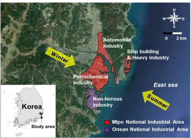
The study area is Ulsan, which is a representative industrial city located in southeastern Korea. A large industrial area including (1) Ulsan and Mipo and (2) Onsan National Industrial Complex is located in east and southeast Ulsan. They are comprised of an automobile, non-ferrous metal, shipbuilding & heavy metal, and petrochemical industrial complex. There are several studies have reported the level and characteristics of the PAHs and halo-PAHs depending on the seasonal wind (Choi et al., 2012; Nguyen et al., 2020; Vuong et al., 2020). These studies reported that non-ferrous, petrochemical, and automobile industrial activities were the dominant sources of PAHs in the atmosphere.
Figure 4.Industrial areas and wind direction as seasonal in Ulsan.
The purpose of this study was to investigate the level of air concentrations depending on seasonal and spatial variation of pPAHs, NPAHs, and OPAHs using PUF-PASs in Ulsan. Second, it is to identify source-receptor relationships on target compounds through diagnostic ratio and correlation analysis.
Finally, it is to assess cancer risk induced by exposure to the target compounds via inhalation and then compare by spatial.
8
Ⅱ. Material and Methods 2.1. Chemicals and material
Target compounds monitored in this study are listed in Figure 2 and Table S1. The native, surrogate, and internal standards of PAHs were purchased from Accustandard (USA), and those of NOPAHs were purchased from Chiron AS (Trondheim, Norway). The surrogate standards include Napthalene- d8, Acenaphthene-d10, Phenanthrene-d10, Chrysene-d12, and Perylene-d12 for PAHs and 1- Nitronapthalane-d7, 2-Nitrofluorene-d9, 9-Nitroanthracene-d9, 3-Nitrofluranthene-d9, and 6- Nitrochrysene-d11 for NOPAHs. S-terphenyl-d14 and 1-Nitropyrene-d9 were respectively used as internal standards for pPAHs and NOPAHs.
9
2.2 Passive air sampling
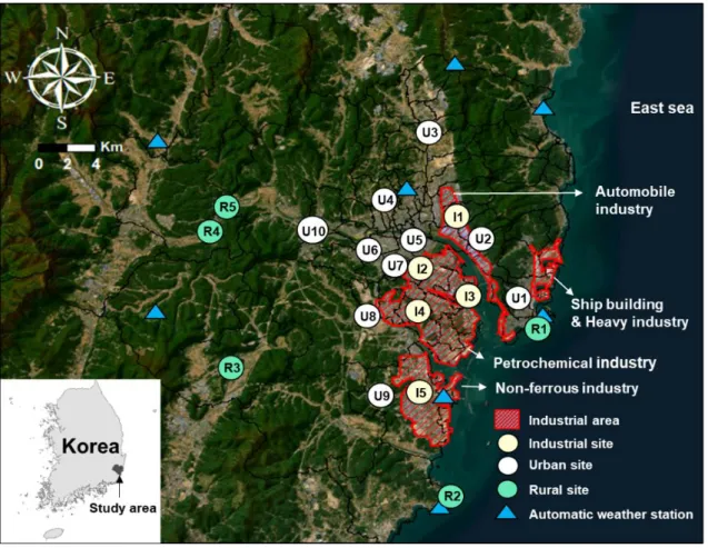
Prior to deployment, the PUF discs were cleaned by sonication using acetone and hexane sequentially for 30 minutes, respectively. To deploy in sampling sites, cleaned PAS-PUFs were wrapped using alumina foil and stored in polyethylene bags. A total of 40 PUF-PASs were deployed in duplicate at every 20 sites consisting of 5 industrial sites, 10 urban sites, and 5 rural sites in Ulsan during the one year from March 2016 to March 2017 (Figure 5). The sampling period can be categorized into 4 seasons: spring (March 22-June 21, 2016, 92days), summer (June 21-September 27, 2016, 99days), fall (September 27-December 27, 2016, 92days), winter (December 27, 2016-March 30, 2017, 94days). Retrieved PUF disks were wrapped using alumina foil and stored at -4 ℃ in a refrigerator until instrumental analysis.
Figure 5. The sampling sites and industrial areas in this study area.
10
2.3 Analysis procedure and instrumental condition
Prior to Soxhlet extraction (20h, 350mL of extraction solvent (n-hexane/acetone = 9:1 (v/v)), surrogate standards were spiked into retrieved PUF disks. The extracts were evaporated up to 1mL using Turbo-Vap II (Caliper, USA) and then transfer the concentrated extract to 10-mL glass tube.
Then each concentrated extract was cleaned up with 70mL of eluent (n-hexane/dichloromethane = 9:1 (v/v)) for PAHs through silica gel columns (bottom and top layer: 2g of sodium sulfate, middle layer:
5g of silica gel).
For NOPAHs, each extract was cleaned up with 70mL of eluent (n-hexane/dichloromethane = 1:9 (v/v)) through silica gel/alumina columns (top layer: 2g of sodium sulfate, middle layer: 5g of alumina, bottom layer: 3g of silica gel). Eluents for PAHs were concentrated up to 500 μL and eluents for NOPAHs were concentrated up to 200 μL using Turvo-Vap and N2 evaporator. Prior to instrument analysis, internal standard (p-terphenyl-d14, 1-nitropyrene-d9) was respectively spiked into all vials for recovery.
In this study, 24 PAHs, 9 OPAHs, and 17 NPAHs were analyzed using GC/MS-EI for PAHs and GC/MS-NCI for NOPAHs. Generally, the concentration of NOPAHs is lower than that of pPAHs;
Thus, GCMS-NCI with high sensitivity for NOPAHs is needed(Galmiche et al., 2021). The chromatograms of the standard and a real sample of NOPAHs analyzed using GC/MS-NCI are indicated in Figure S1. The used column was DB-5MS for all target compounds. Helium (He) gas was chosen as a carrier gas, and methane (CH4) gas was chosen as a reactant gas. The samples were injected at 280℃ and MS was run at 230℃. For PAHs, the GC temperature was initially at 60℃ for 1min, then increased to 260°C as 10 °C/min (5 min). And then increased to 320 as 5 °C/min (3 min).
For NPAHs, the GC temperature was initially at 60℃, then increased to 150°C as 20 °C/min (10 min) and increased to 230 as 10 °C/min (12 min) and increased to 320°C as 30 °C/min (2.5 min)
Figure 6. Gas chromatography/mass spectrometry-negative chemical ionization (GC/MS-NCI)
11
2.4 Quality assurance and Quality controls (QA/QC)
Method blanks consist of field blank and lab blank. Field blanks and lab blanks were collected respectively (n=8 and 9); The blank samples were analyzed using the same procedure used in the real samples. The amount of target compounds is modified using the average of blank samples. The average recovery rates of surrogates for PAHs and NOPAHs were 60% - 97% and respectively expressed in Table 2. Method detection limits (MDL) were carried out using following equation 1.
𝑀𝐷𝐿 = 𝑡𝑆× 𝑆𝑇𝐷 (1) ts : The student’s t value for 99% confidence level
STD: The standard deviation of 7 replicate spiked samples.
Instrumental detection limit (IDL) is considered as three times the standard deviation of the noise level.
Table 2. Recovery rate of surrogates
Surrogate standards Recovery Internal standards
PAHs
Phenanthrene-d10 60%
S-terphenyl-d14
Chrysene-d12 96%
Perylene-d12 87%
NOPAHs
1-Nitronapthalane-d7 74%
1-Nitropyrene-d9
2-Nitrofluorene-d9 89%
9-Nitroanthracene-d9 65%
3-Nitrofluranthene-d9 68%
6-Nitrochrysene-d11 71%
12 Table 3. MDL and IDL for target compounds.
Compounds IDL MDL Compounds IDL MDL
PAHs (ng) NPAHs (ng)
Nap 0.119 5.333 1-NNap 0.038 1.794
Acy 1.094 4.046 2-NNap 0.077 2.092
Ace 0.373 4.011 5-NAce 0.563 1.751
Flu 0.684 6.328 2-NFlu 0.194 1.617
Phe 0.166 4.405 9-NAnt 0.600 5.906
Ant 0.985 4.258 3-NPhe 0.640 7.907
Flt 2.793 5.543 9-NPhe 0.654 7.527
Pyr 2.833 7.338 2-NFlt 0.509 2.321
BcP 2.373 2.835 3-NFlt 0.362 2.060
BaA 1.202 5.373 1-NPyr 0.061 3.875
Chr 0.796 3.734 4-NPyr 0.064 1.163
B[b+j]F 6.616 3.137 2-NPyr 0.138 0.966
BkF 1.193 4.021 7-NBaA 0.277 3.914
7,12-DMBaA 0.301 4.265 6-NChr 0.534 3.060
BeP 1.268 5.156 1,6-DNP 0.177 4.691
BaP 1.441 3.070 1,3-DNP 0.224 3.692
3-MCA 1.669 1.861 1,8-DNP 0.249 3.029
IcdP 1.112 4.410 OPAHs (ng)
DBahA 1.150 2.515 1,4-NAQ 0.073 1.129
BghiP 1.097 5.316 1-NAD 0.125 0.912
DBaiP 2.873 4.817 9-FLO 0.087 6.471
DBahP 4.118 2.981 XAT 0.116 0.569
DBalP 3.277 1.921 ANQ 0.274 2.220
MANQ 0.100 0.808
BaFL 0.037 0.770
BENZ 0.099 2.209
BaAD 0.073 2.322
13
2.5 Calculation of PAHs concentration in air
Using passive air samplers, the flow rate is not measured separately; thus, only the sequestered amount on the PUF disk (CPUF: ng) can be obtained. Therefore, the air concentration of target compounds (CAir: ng/m3) need to calculate using below the equation 2 with amount of sequestered on PUF disk (ng/PUF), the sampling days, and the sampling rate of passive air samplers (Rs: m3/day).
𝐶Air= 𝐶PUF
𝑅s×𝐷s (2) Where, Ds represents the sampling days. In the previous studies, a same average sampling rate which is 4.0 - 5.0 m3/day was applied for each target compound at all sites(Harner et al., 2013; Jariyasopit et al., 2019; Vasiljevic et al., 2021). However, the sampling rate is different depending on the meteorological conditions and physicochemical characteristics of target compounds. The global atmospheric passive sampling network developed a new prediction model of sampling rate using a MATLAB code with meteorological data (temperature, pressure, wind speed, wind direction, and relative humidity) and the physicochemical properties (MW: molecular weights, KOA: Octanol-air partition coefficient, and UOA: internal energy of transfer)(Herkert et al., 2016; Herkert et al., 2018).
These properties are listed in Table S1. MATLAB code can estimate each sampling rate (Rs) and an effective sampling volume (Veff) as to a specific compound and specific sampling location, respectively. Finally, the air concentration was calculated by below equation 3.
𝐶Air= 𝐶PUF
𝑉eff (3)
14
2.6. Meteorological and criteria/hazardous air pollutant data
Meteorological data (temperature, pressure, wind speed, wind direction, and relative humidity) from one automated synoptic observing system (ASOS) and 7 automatic weather stations (AWSs) were provided from Korea meteorological administration (KMA, http://www.data.kma.go.kr/). Wind fields were drawn as seasonal using the CALMAET meteorological model (TRC Companies, USA).
Criteria air pollutant data (e.g., SO2, NO2, O3, CO, PM10, and PM2.5) from thirteen stations were provided from the Air Korea (https://www.airkorea.or.kr). Hazardous air pollutants (HAPs) were provided from two hazardous air pollutants monitoring networks.
2.7 Statistical tools
Statical tools were used for the interpretation of data distribution and relationship. Shapiro-Wilk normality test, Pearson, and Spearman correlation analysis were performed using SPSS statistics version 20.0 (IBM, USA) to investigate data distribution and correlation between data set. Mann- Whitney rank sum test was conducted using SigmaPlot version 12.0 (Systat Software Inc., USA) to investigate the statistically significant difference between data set.
2.8 Risk assessments
The potential cancer risk caused via inhalation of PAHs and NPAHs was assessed using the model of incremental lifetime cancer risk (ILCR). Before calculating ILCR, measured concentrations were converted the BaPeq concentration based on the toxicity equivalence factor (TEF) of PAHs and NPAHs.
𝑇𝐸𝑄 = ∑𝐵𝑎𝑃𝑒𝑞= ∑𝐶𝑖× 𝑇𝐸𝐹𝑖
Where, TEQ is toxic equivalent concentration, Ci is a concentration of an individual compound, TEFi
is the toxic equivalent factor of an individual compound. TEF values are listed in Table 4. The total of BaP equivalent (BaPeq) concentrations of individual compounds was used as input data in the equation of ILCR. The ILCR equation is below.
𝐼𝐿𝐶𝑅 = (𝐼𝑆𝐹 × 𝐵𝑎𝑃𝑒𝑞× 𝐼𝑅 × 𝐸𝐹 ×ED× 𝑐𝑓)/(𝐵𝑊 × 𝐴𝑇)
Where, ISF is inhalation slope factor (mg/kg/day), IR is inhalation rate (m3/h), EF is exposure frequency (day/year), ED is exposure duration (year), cf is conversion factor (10-6), BW is body weight and AT is averaging time (days). The potential cancer risks of target compounds were compared to an acceptable level by US-EPA. These values are generally recognized as acceptable levels when below 10-6 and serious levels which caused cancer risk possible above 10-6 for possibly caused cancer risk(Fewtrell & Bartram, 2001).
15 Table 4. Toxic equivalent factors of PAHs and NPAHs
PAHs TEFi NPAHs TEFi
Flu 0.001* 5-NAce 0.03b
Phe 0.001* 2-NFlu 0.01a
Ant 0.01* 9-NAnt 0.0032a
Flt 0.001* 2-NFlu 0.0026a
Pyr 0.001* 1-NPyr 0.1c
BaA 0.1* 6-NChr 10a
Chr 0.01*
BbF 0.1*
BjF 0.1**
BkF 0.1*
DMBA 21.8**
BaP 1*
3MCA 1.9**
Incd 0.1*
DahA 1*
B[ghi]P 0.01* DbaiP 10**
DbahP 10**
DbalP 10**
*TEFi was provided from US-EPA (2010)
**TEFi was provided from OEHHA (1994)
aTEFi was provided from Yadav and Devi (2021)
bTEFi was provided from Lixin et al. (2020)
cTEFi was provided from Hao et al. (2018)
16
Ⅲ. Results and Discussion
3.1. Calculation of sampling rates
Prior to concentration calculation, the average sampling rates from each AWS site were calculated and these results were interpolated using ArcGIS version 10.4.1 (Inverse distance weighting: IDW) (Figure 7). The calculated average sampling rates were extract using selection location method at ArcGIS and then these results were interpolated using IDW. Through this method, sampling rates of each site and compound were calculated and then applied to calculate air concentration of target compound, respectively. This method can prevent the air concentration would be underestimated and overestimated compared to applying the sampling rate as a specific value.
Figure 7. The method of calculation on average sampling rate.
17
3.2. Level of concentration of target compounds
The range of detection ratio for PAHs is 5% (DBalP, DBahP)-100%, but 7,12-DMBaA and 3-MCA were not detected in this study. For NPAHs, the range of detection ratio is 3%(6-NChr)-100%, and isomers of dinitropyrene were not detected. Meanwhile, all OPAHs were detected in all samples. The average concentrations of individual target compounds (PAHs, OAPHs, and NPAHS) were shown in Figure 8. The LMW compounds were more detected than HMW compounds because PUF-PAS could be more accumulated to highly volatile compounds than less-volatile compounds. The abundant compounds were orderly Phe, Flt, Pyr, Flu, and Ant for PAHs, 9-FLO, ANQ, XAT, and NAD for OPAHs, 1-NNap, 2-NNap, 9-NAnt, 2+3-NFlt for NPAHs. These compounds are low and medium molecular weights having 2-, 3-, and 4-ring. This profile of concentration on PAHs is similar to previous studies in Ulsan(Choi et al., 2012; Vuong et al., 2020).
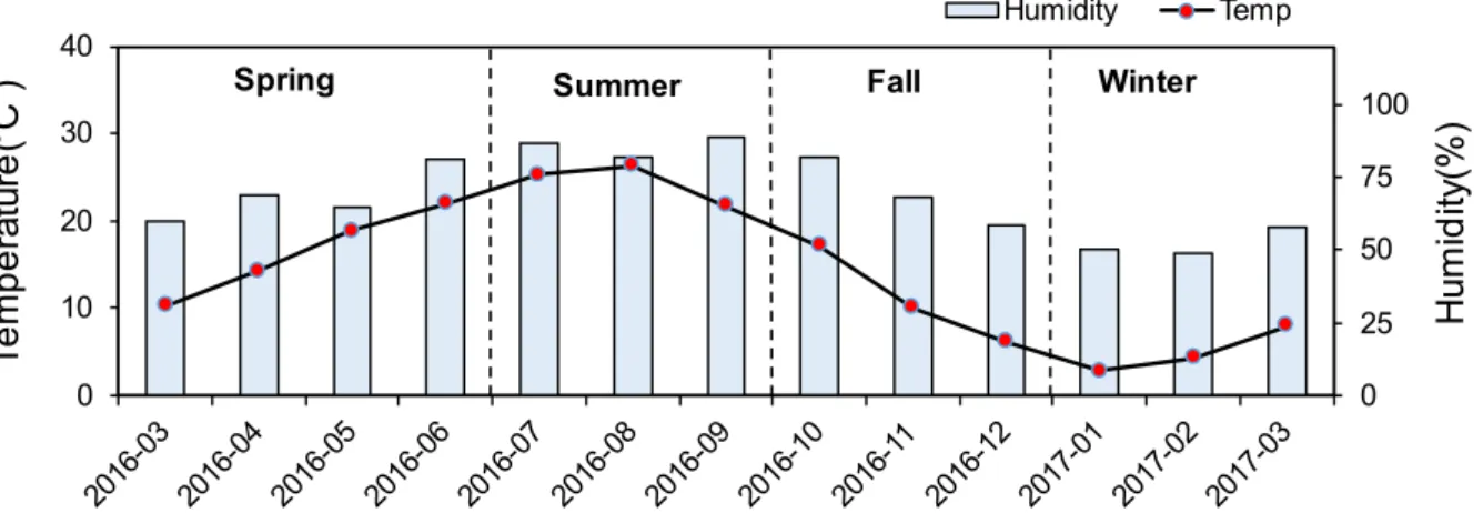
Figure 9 shows the seasonal concentration of PAHs, OPAHs, and NPAHs. The average concentration of PAHs, OPAHs, and NPAHs is similar compared to other studies (Table S2). The average concentration of PAHs showed the highest in fall (18.11±7.28 ng/m3), followed by winter (14.69±7.01 ng/m3), spring (13.13±6.61 ng/m3), and summer (10.79±5.14 ng/m3). Herein, the concentration of PAHs in the fall was statically higher than summer season (Rank sum test: p<0.01). And fall and winter seasons have significantly high concentrations than spring and summer, respectively (Rank sum test: p<0.05). Generally, the concentration of PAHs is higher in winter than in other seasons because the mixing layer is lower than in other seasons, combustion of heating, biomass burning, and can be affected by long-range transport by northwest wind(Lee & Kim, 2007; Ma et al., 2010; Nguyen et al., 2020). However, the concentration of PAHs was higher in the fall than in winter, which is believed to be due to overlapping sampling periods and each season. Figure 10 shows the concentration of PAHs provided by the hazardous atmosphere monitoring station during the same sampling period in this study. The concentration of PAHs was the highest during November and December which is the sampling period for fall samples. Even during the winter sampling period, the concentration of PAHs also decreases dramatically as the temperature increases in March (Figure 11).
Additionally, the concentration of PAHs in fall seemed higher than in winter, but there was no statistically significant difference. The seasonal concentration of OPAHs is indicated in Figure 9. In the case of OPAHs, the average concentration is highest in winter (3.78±2.63 ng/m3), by followed fall (3.60±1.90 ng/m3), summer (3.41±2.22 ng/m3), and spring (2.01±1.30 ng/m3). However, except for the spring, it seems to be no difference in the concentration of OPAHs by season. Also, there was no statistically significant difference. Unlike PAHs, the concentration of OPAHs was not decreased in summer, suggesting that OPAHs were formed through the secondary formation. Among them, ANQ increased in summer compared to other seasons. The concentration of ANQ was highest at 1.39 ng/m3
18
(41%) in the summer, followed by winter (1.27 ng/m3, 34%), fall (0.70 ng/m3, 19%), and spring (0.54 ng/m3, 27%). The reason for the secondary formation of ANQ is discussed in more detail in section 3.4. For NPAHs, the order of higher seasonal average concentration is by following fall (193.78±88.82 pg/m3), winter (156.65±62.83 pg/m3), summer (150.43±54.69 pg/m3), and spring (137.67±51.07 pg/m3). Generally, NPAHs are formed through direct emission sources with parent PAHs or secondary formations like photochemical reactions(Kojima et al., 2010). In this study, NPAHs could be heavily influenced by direct emissions with pPAHs in the fall, while secondary formation might have been influenced in the summer.
Figure 12 shows the fraction of PAHs, OPAHs, and NPAHs, indicating that PAHs having 3 rings and 4 rings contribute to a fraction of more than 95%. OPAHs with three rings are mainly present throughout the four seasons. Especially, OPAH with two rings was hardly detected in winter. In the case of NPAHs, there was no clear difference between seasons.
Figure 8. The level of PAHs, OPAHs, and NPAHs in this study.
Figure 9. Boxplot of seasonal concentrations of a) PAHs, b) OPAHs, and c) NPAHs.
19
Figure 10. Average concentration of PAHs monthly at hazardous air pollutant stations.
Figure 11. Average monthly temperature and humidity at ASOS station.
20 Figure 12. Seasonal fraction and concentration of PAHs, OPAHs, and NPAHs.
21
3.3. Spatial distribution
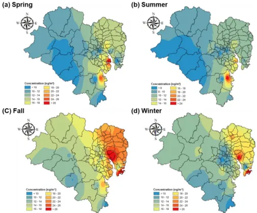
Spatial distributions of PAHs, OPAHs, and NPAHs as seasonal are presented in Figure 13-15, and wind fields as indicated in Figure 16. Spatial distributions of PAHs were similar, respectively, between spring and summer, autumn and winter. PAHs seem to have been mainly affected by non- ferrous metal and petrochemical industrial complexes, respectively in the spring and summer. On the other hand, in the fall and winter, PAH concentrations were higher near the automobile industrial complex than near the petrochemical and non-ferrous industrial complexes. To interpret the spatial distribution of PAHs, it was compared with the seasonal wind field. The wind fields showed mainly to exist east wind in spring and summer, and the north and northwest winds mainly blew in fall and winter. In Ulsan, when the east wind blows in warm seasons, it is greatly affected by the petrochemical complex and when the northwestern or north wind blows in the cold season, it is affected by the automobile industrial areas. In fall and winter, high concentrations are shown in the R1 area, which is far from the influence of the automobile industrial complex. This phenomenon can be explained by the wind fields and average sampling rates. (Figure 7) When the main wind direction of the cold season is northwest wind, it is affected by automobile industrial complex emissions, and the average sampling rate is lower than in other regions due to differences in weather conditions. Thus, it can be interpreted that high concentrations of PAHs are detected by accumulating more PAHs in PUF.
OPAHs have a spatial distribution very similar to that of pPAHs in spring, fall, and winter. However, high concentrations of OPAHs were found in automobile industrial complexes in the summer, and the impact of petrochemical complexes also appeared to be increased. Compared to PAHs, the effect of non-ferrous metal complexes seems to be relatively small. As a result, OPAHs seem to be greatly affected by the automobile industrial complex. Except for summer, NPAH shows high concentrations not only in all industrial areas but also in urban areas with high population density (Figure S3).
NPAHs seem to be mainly affected by both petrochemical and non-ferrous metal industrial activities in summer. In particular, a high concentration of NPAHs was observed at U06 site in winter, meanwhile, PAHs and OPAHs showed low concentrations here. Among NPAHs, 9-NAnt has indicated the highest concentration in winter. In previous studies, 9-NAnt was mainly observed in diesel emissions and diesel standard reference material (SRM) and can be also formed through the heterogeneous reaction of anthracene bounded to particles with nitrate(Bamford & Baker, 2003; Fox
& Olive, 1979; Paputa-Peck et al., 1983; Pitts Jr et al., 1978). Therefore, it seems to be greatly influenced by diesel engines as an area with a lot of traffic. Unlike pPAHs, in the case of NPAHs, it is difficult to separate specific emission sources due to the coexistence of the influence of the primary emission and secondary formation of the industrial complex rather than the influence of the seasonal wind direction
22
Figure 13. Spatial distribution of PAHs in Ulsan, in (a) spring, (b) summer, (c) fall, and (d) winter.
Figure 14. Spatial distribution of OPAHs in Ulsan, in (a) spring, (b) summer, (c) fall, and (d) winter.
23
Figure 15. Spatial distribution of NPAHs in Ulsan, in (a) spring, (b) summer, (c) fall, and (d) winter.
Figure 16. Wind field in Ulsan, in (a) spring, (b) summer, (c) fall, and (d) winter.
24
3.4. Source identification 3.4.1 Correlation analysis
Correlation analysis was performed to investigate not only the relationship between criteria air pollutants and NOPAHs but also the relationship between parent molecules and derivative molecules.
The results of the correlation analysis are presented in Table 5-6, S3-9. The individual PAHs showed a significant positive correlation with individual OPAHs and NPAHs, which are believed to have been affected by similar sources between pPAHs and derivates PAHs. NO2 and O3 are known as the main atmosphere oxidant agents in the secondary photochemical reaction of NOPAHs(Zeng et al., 2020).
Therefore, the relationship between oxidant agents and NOPAHs is important to understand the formation mechanism of NOPAHs. Except for NAQ, NAD, and 9-FLO, the others OPAHs substances showed a statistically significant negative correlation with NO2. In the previous paper, it is suggested OPAHs are related to secondary formation when they have a negative correlation with NO2
(Wnorowski & Charland, 2017). In the study, it obtained similar results suggesting that OPAHs are not only primarily generated like PAHs, but also OPAHs are formed by secondary formation through a reaction between the emitted parent molecules and atmospheric oxidants. 9-FLO has a significantly negative correlation with O3, but it has a significantly strongly positive correlation with PAHs. In the previous studies, 9-FLO had higher concentrations in both gas and particulate phases in ozone-free environments(Albinet et al., 2007; Nocun & Schantz, 2013). It can be inferred that the reaction between 9-FLO and ozone is an elimination pathway. The ratios of 9-FLO/Flu in each season and site were around 1 (Figure 17). However, this ratio was high in the U1 site in summer, and the concentration of O3 was also high. it can be inferred to form 9-FLO from the oxidative transformation by O3. The ratio of ANQ/ANT is higher than 1 in all samples (Figure 19). Especially, the ratio is higher in summer than in other seasons. The ratio above 1 suggests ANQ formed from ANT(Awonaike et al., 2021). It can be interpreted as ANQ may be formed by the transformation of ANT. However, ANQ has a positive correlation with other primary pollutants. It can be implied that OPAHs can be emitted from similar emission sources with PAHs or also formed through secondary formation. For this reason, the concentration of OPAHs seems to be high even in summer.
In the case of NPAHs, 5-NAce and 7-NBaA show positive correlations with primary pollutants and parent PAHs, which means they were discharged from primary pollutants. Previous studies reported that 5-NAce is emitted by vehicle emission(Alves et al., 2016), coal combustions(Huang et al., 2014), and biomass burning(Vicente et al., 2016) and 7-NBaA is emitted by diesel exhaust(Chiu & Miles, 1996; Nielsen et al., 1984). However, 1-NNap and 2-NNap show negative correlations with NO2, it is suggested possible secondary formation.
25 Table 5. Result of correlation analysis between NPAHs and CAPs.
Table 6. Result of correlation analysis between OPAHs and CAPs.
26
Figure 17. Ratio of 9-Fluorenone/Fluorene at each sampling site
Figure 18. Ratio of 7,12-Benz[a]anthracenedione /Benzo[a]anthracene at each sampling site.
Figure 19. Ratio of 9,10-Anthracenedione/Anthracene at each sampling site
27
3.4.2 Diagnostic ratio
Diagnostic ratios represent the ratio of individual compounds with known emission sources, potential emission sources can be characterized as a range of ratios. The diagnostic ratio was calculated to find the potential emission sources of PAHs by land use and season. The ratios of Flt/(Flt+Pyr) and IcdP/(IcdP+BghiP) were used to identify the origin of combustion. For IcdP/(IcdP + BghiP), a ratio below 0.2 means probably contributed from unburned petroleum, between 0.2 and 0.5 implies liquid fossil fuel, and the ratio above 0.5 suggested a grass/wood/coal combustion origin(Yunker et al., 2002). For Flt/(Flt+Pyr), a ratio below 0.5 means petrogenic sources while a ratio above 0.5 suggested a grass/ wood/coal combustion origin(Yunker et al., 2002). The ratio of Flu/(Flu+Pyr) is also used to identify the emission source whether petrogenic or pyrogenic. It is implied to the emission source is petroleum when the ratio is below 0.5. On the other hand, a ratio above 0.5 means that the emission source is coal and biomass burning(Guo et al., 2010; Qiao et al., 2006). In Figure 20, Flt/(Flt+Pyr) and Flu/(Flu+Pyr) were expressed on the scatter plot to understand the characteristics of seasonal emission sources. The scatter plot implied PAHs in spring and summer originated from petroleum sources. In fall and winter, PAHs might be emitted from not only petrogenic combustion but also biomass and coal combustion. Figure 21 was drawn with Flu/(Flu+Pyr), and IcdP/(IcdP + BghiP) by land-use and season. There was no difference in emission sources by each land use. Ulsan seems to be influenced by different emission sources as seasonal. It seems to be influenced by unburned petroleum and liquid fossil fuel combustion in spring and summer, and mainly by liquid fossil fuel combustion and glass/wood/coal combustion in autumn and winter.
Figure 20. Scatter plot of two diagnostic ratios of Flt/Flt+Pyr and Flu/Flu+Pyr.
28
Figure 21. Two-scatter plots of two diagnostic ratios of Flu/Flu+Pyr and IcdP/IcdP+BghiP by season and land-use.
In the case of NPAHs, the diagnostic ratio was identified to determine the effects of primary emission and secondary formation. The ratio of 1-NNap/2-NNap is used to identify whether it is reacted by OH radicals or nitrate(Sasaki et al., 1997). A ratio above 2 suggests the formation reaction occurs by the dominance of the nitrate. Meanwhile, A ratio less than 2 means the formation reaction occurs by the dominance of the OH radicals. In Figure 22, most of the sites have lower than 2 suggesting that nitronaphthalene might be formed by secondary formation by reaction with OH radicals. However, it shows a value of more than 2 in the fall and winter at the U10 site. Compared to the spatial distribution of NO2 and the ratio of 1-NNap/2-NNap, the highest concentration of NO2 was observed at U10. It suggests that nitronaphthalene may have reacted with nitrate to form a secondary product.
The following diagnostic ratio was 2+3-NFlt/2-NPyr which is used to identify secondary formation pathways(Chuesaard et al., 2014; Zielinska et al., 1989). A ratio close to 100 suggests the dominant reaction with nitrate during nighttime meanwhile, a ratio less than 10 means the dominant reaction with OH radicals during daytime(Y. Zhang et al., 2018). In figure 23, the ratios of 2+3-NFlt/2-NPyr were less than 10 at most of the samples. It suggests NPAHs might have formed via OH radical- initiated reaction in the daytime. The following diagnostic ratio was 2+3-NFlt/1-NPyr which is known that the effect of the secondary formation when the ratio is higher than 5, the effect of primary emission is clear when the ratio is lower than 5(J. Zhang et al., 2018b). In Figure 24, it shows the ratios were higher than 5 at most of samples. Except for a few samples at urban sites in the spring, it implies that NPAHs are primarily formed by secondary formation.
29 Figure 22. Diagnostic ratio of 1-NNap/2-NNap.
Figure 23. Diagnostic ratio of 2+3-NFlt/2-NPyr.
Figure 24. Diagnostic ratio of 2+3-NFlt/1-NPyr.
30
3.5 Risk assessment
BaPeq was calculated with individual concentrations and toxic equivalent factor (TEFi). The averages of fraction and TEQ were expressed by seasonal (Figure 25). The average of TEQ shows highest in winter (0.378 ng-TEQ/m3), followed by spring (0.376 ng-TEQ/m3), fall (0.337 ng-TEQ/m3), and summer (0.229 ng-TEQ/m3). There was no difference between each season except for summer. In terms of fraction, PAHs not listed in EPA had high portion, followed by 13 PAHs listed by US-EPA and ∑NPAHs. NPAHs contributed relatively low to the TEQ about 1-2% due to the low concentration.
However, it should not be overlooked because NPAHs did not have many toxicological studies yet compared to PAHs, so most NPAHs do not have TEF values. Even OPAHs also do not have available toxicity coefficient values.
Figure 25. (a) Fraction and (b) Toxic equivalent concentration (TEQ) by seasonal.
Figure 26. Stack bar of the total incremental lifetime cancer risk (ILCR) of PAHs and NPAHs.
31
The potential cancer risk was assessed using the model of incremental lifetime cancer risk (ILCR).
The seasonal averages of ILCR were drawn in Figure 26 and listed as winter (6.799E-08), spring (6.513E-08), fall (5.710E-08), and summer (2.215E-08) in the order of seasonal high risk. The average risk at all seasons in Ulsan was lower than the US EPA (1.0E-06 or 1.0E-04) and WHO (1.0E- 05) risk criteria. Therefore, it seems to be a safe level.
In order to understand the spatial distribution of cancer risk, the ILCR values of PAHs and NPAHs calculated for each site were interpolated using inverse distance weights (IDW) in ArcGIS (Figure 27- 28). For PAHs, the cancer risks were high in nonferrous metal industrial areas and petrochemical industrial areas in spring and summer. Compared to the spatial distribution of PAHs concentration, the pattern was quite similar. However, PAHs concentrations were low at the U3 site, but the risk was high in the spring. Non-ferrous metal complexes (I5) and petrochemical complexes (I2 and I3) have a high risk the damage to local residents is small due to their low population density. However, the area having higher levels of risk moved to near the automobile industrial area (U2) in fall and winter. In terms of NPAHs, the spatial distribution of cancer risk was slightly different from PAHs. The impact of the automobile industrial complex was hardly seen, and the impact of the non-ferrous metal industrial complex (I5) was clearly confirmed. It suggests that NPAHs having TEFi were related to industrial activity from the non-ferrous metal industrial area.
32
Figure 27. Spatial distribution of the total incremental lifetime cancer risk (ILCR) for PAHs.
Figure 28. Spatial distribution of the total incremental lifetime cancer risk (ILCR) for NPAHs.
33
Ⅳ. Conclusion
This is the first study that investigated PAHs, NPAHs, and OPAHs together using passive air samplers in Korea. In this study, the levels of each target compound were investigated by 20 sites. The average concentration of PAHs, OPAHs, and NPAHs was similar with previous studies. Low molecular weight (LMW) and middle molecular weight (MMW) compounds having 2-, 3-, and 4- aromatic benzene rings were mainly detected, meanwhile high molecular weight (HMW) compounds having 4-, 5-, and 6-rings (7,12-DMBaA, 3-MCA, 1,6-DNP, 1,3-DNP, and 1,6-DNP) were not detected. In terms of seasonal variation, the concentration of PAHs is highest in fall by following winter, spring, and summer. On the other hand, NOPAHs were not influenced by significant seasonal changes due to the secondary formation during the summer. In terms of spatial distribution, PAHs were greatly influenced by the non-ferrous metal industrial complexes and petrochemical industrial complexes when the east wind blew during the warm seasons, but the impact of the automobile industrial complex was clearly identified as evidence of potential emission sources during the cold season that blew northwest wind. In particular, OPAHs were greatly influenced by automobile industrial complexes while the impact of nonferrous metal complexes decreased. However, there is no specific potential emissions sources of NPAHs. Because they were simultaneously affected by primary emission and secondary formation.
The relationship between target compounds and CAPs was identified through correlation analysis.
There was a high correlation between parent PAHs and derivates PAHs, which were expected to have similar potential emission sources. However, NO2 and some NOPAHs show a negative correlation, suggesting the possibility of secondary formation. The emission sources and formation pathways of PAHs and NPAHs were investigated using the diagnostic ratio. As a result of diagnostic ratio, NPAHs were mainly formed via secondary formation with OH radicals during the daytime. In the case of PAHs, it was confirmed that they were mainly affected by liquid fossil fuel combustion, greatly influenced by petroleum evaporation in warm seasons, and greatly influenced by biomass burning and coal combustion in cold seasons.
The potential cancer risk was evaluated by the model of ILCR and was not higher than the criteria of UEA-EPA in all samples. Not listed PAHs contributed to the high portion of cancer risk, meanwhile NPAHs contributed to just 1%. However, derivate PAHs should not be overlooked because the available toxicity coefficients are limited. The spatial distribution of PAHs and NPAHs was confirmed using the ILCR value calculated at each sampling site, respectively. It showed some different tendencies compared to the spatial pattern of concentration. In the case of PAHs, high risk was identified in the U4 area, where the concentration was low. It needs to control PAHs because this site
34
is high population density than an industrial area. For NPAHs, high risk was identified especially in non-ferrous metal industrial complexes suggesting that NPAHs having toxic coefficients were emitted in non-ferrous metal industrial complexes.
In this study, the seasonal and spatial variation were confirmed to identify the level of target compounds (PAHs, OPAHs, and NPAHs) and their potential emission sources using PAS-PUF in Ulsan, which is large industrial area. These results can be used as basic data for domestic NOPAHs research in the future. However, long-term monitoring is required to clearly identify the emission source of contamination. Since PAS-PUF mainly collects gas phases, there are limitations in using diagnostic ratio and identification of long-range transport. To solve these limitations, it is necessary to predict the particulate concentration with gas-particle partitioning and correct the concentration.
Further studies on particulate NOPAH using an active air sampler are also necessary to clearly identify gas-particle distribution on NOPAHs in Korea.
35
Reference
Albinet, A., Leoz-Garziandia, E., Budzinski, H., & Viilenave, E. (2006). Simultaneous analysis of oxygenated and nitrated polycyclic aromatic hydrocarbons on standard reference material 1649a (urban dust) and on natural ambient air samples by gas chromatography-mass spectrometry with negative ion chemical ionisation. J Chromatogr A, 1121(1), 106-113. https://doi.org/10.1016/j.chroma.2006.04.043 Albinet, A., Leoz-Garziandia, E., Budzinski, H., & Viilenave, E. (2007). Polycyclic aromatic
hydrocarbons (PAHs), nitrated PAHs and oxygenated PAHs in ambient air of the Marseilles area (South of France): concentrations and sources. Sci Total Environ, 384(1-3), 280-292. https://doi.org/10.1016/j.scitotenv.2007.04.028
Albinet, A., Leoz-Garziandia, E., Budzinski, H., Villenave, E., & Jaffrezo, J. L. (2008).
Nitrated and oxygenated derivatives of polycyclic aromatic hydrocarbons in the ambient air of two French alpine valleysPart 1: Concentrations, sources and gas/particle partitioning. Atmospheric Environment, 42(1), 43-54.
https://doi.org/10.1016/j.atmosenv.2007.10.009