Share repurchases as a potential tool to mislead investors

(1)

Share repurchases as a potential tool to mislead investors☆

Konan Chan

^a

, David L. Ikenberry

^b,

⁎ , Inmoo Lee

^c

, Yanzhi Wang

^d

aSchool of Economics and Finance, University of Hong Kong, Hong Kong

bDepartment of Finance, University of Illinois at Urbana-Champaign, Champaign, Illinois 61821, USA

cDimensional Fund Advisors, Austin, Texas 78746, USA

dDepartment of Finance, Yuan Ze University, Jung-Li 320, Taiwan

a r t i c l e i n f o a b s t r a c t

Article history:

Received 16 July 2008

Received in revised form 16 October 2009 Accepted 16 October 2009

Available online 28 October 2009

A rich literature argues that stock repurchases often serve as positive economic signals beneficial to investors. Yet due to their inherentflexibility, open-market repurchase programs have long been criticized as weak signals lacking commitment. We evaluate whether some managers potentially use buyback announcements to mislead investors. We focus on cases where managers were seemingly under heavy pressure to boost stock prices and might have announced a repurchase only to convey a false signal. For suspect cases, the immediate market reaction to a buyback announcement does not differ from that generally observed. However over longer horizons, suspectfirms do not enjoy the improvement in economic performance otherwise observed. Suspectfirms repurchase less stock. Further, managers in suspectfirms have comparatively higher exposure to stock options, a potentially endogenous result suggesting greater sensitivity to both stock valuation and to future equity dilution. Overall, the results suggest only a limited number of managers may have used buybacks in a misleading way as“cheap talk.”Yet as theory also suggests, wefind no long-run economic benefit to this behavior.

JEL classiﬁcation:

G30 G35 Keywords:

Share repurchase Earnings management Managerial signal

1. Introduction

Many studies consider the potential economic value of a stock repurchase and the reasons why company executives might wish to engage them. A well-developed literature documents that shareholders have historically realized positive abnormal returns subsequent to a repurchase announcement, indicating at least some economic beneﬁt on average. On the other hand, open-market stock repurchase programs (OMSRs) have long been criticized for lacking credibility as a quality signal (e.g.,Vermaelen, 1981;

Comment and Jarrell, 1991). Compared toﬁxed-price buyback methods, open-market buyback programs are simply authorizations, not commitments, which permit management to repurchase stock at their whim, if at all. The concern is that open-market authorizations pose few barriers to managers who might wish to engage in mimicking behavior. Reporting and disclosure requirements surrounding actual transactions are minimal in the U.S. and these authorizations, at their initiation, impose few costs or limitations on the company or its management. Further, managers have historically not borne any reputational penalty for announcing and then failing to buy back stock.

☆ Chan acknowledgesfinancial support from the National Science Council of Taiwan (NSC92-2416-H-002-049-EF). Lee acknowledgesfinancial support from the Ministry of Education of Singapore (R-315-000-059-112). We acknowledge useful comments from Sheng-Syan Chen, Yehning Chen, Joseph Fan, Yaniv Grinstein, Shing-Yang Hu, Charlie Kahn, K.C. John Wei, Michael Weisbach, T.J. Wong, Hua Zhang, and the seminar participants at Chinese University of Hong Kong, Concordia University, Korea Advanced Institute of Science and Technology, Michigan State University, National Taiwan University, National University of Singapore, Vanderbilt University, the University of Hong Kong, the University of Virginia, The 2005 HKUST Finance Symposium, and The 2006 Annual American Finance Association meetings. This paper was initiated while Konan Chan was at National Taiwan University and largely completed while Inmoo Lee was at the National University of Singapore. The views in this paper are those of the authors but not of Dimensional or its affiliates.

⁎Corresponding author. Tel.: +1 217/333 6396; fax: +1 217/333 4101.

E-mail addresses:[email protected](K. Chan),[email protected](D.L. Ikenberry),[email protected](I. Lee),[email protected](Y. Wang).

doi:10.1016/j.jcorpﬁn.2009.10.003

Contents lists available atScienceDirect

Journal of Corporate Finance

j o u r n a l h o m e p a g e : w w w. e l s e v i e r. c o m / l o c a t e / j c o r p f i n

(2)

Given this lack of downside penalty or risk, an interesting empirical question is whether, among the general population of buybacks, a subset of cases exists where the evidence might suggest that managers announced open-market buyback programs with the intent of misleading investors. Given that executive compensation is often highly linked tofirm value, these managers would seemingly face strong incentives to boost stock prices.Fried (2005)raises the notion that open-market share repurchases (OMSR) could be used as a false-signaling device. Even though one expects natural market mechanisms and government regulation to prevent managers from sending false signals, there is anecdotal evidence of managers taking advantage of regulatory loopholes within or outside legal boundaries. Many academic papersfind that managers seem to engage in stock price manipulation prior to important corporate events (e.g., annual meetings (Dimitrov and Jain, 2008) and equity offerings (Teoh et al., 1998)). Moreover,Bhojraj et al. (2009)find that low earnings qualityfirms which beat analyst forecasts, even marginally, enjoy short-term stock price benefits by cutting discretionary expenditures. A recent paper byPeng and Roell (2008)provides a theoretical perspective of this type of behavior and how stock based compensation can lead managers to engage in costly, short-term price manipulation.

Of course, no pure, ex-ante measure of managerial intent exists. Whatever measure we might develop will, at best, be an indirect, noisy proxy. One indirect proxy that might readily be considered is program size; larger programs are uniformly viewed in the literature as stronger signals (e.g.,Comment and Jarrell, 1991). This is particularly true offixed-price programs where markets can generally rely on managers to follow through and where credibility of the program is generally not questioned. While there is ample evidence that markets do initially react more favorably to larger open-market buyback programs, program size, regrettably, is not a convincing or a compelling measure of managerial intent. Because of the inherentflexibility of open-market repurchases, managers have the freedom to set program size irrespective of whatever true intention they might have.¹Firms can and do initiate programs even if they have no immediate intention of buying back stock.²Further, managers who do not wish to overtly signal the market can“hide”a large buyback program by executing a series of smaller programs in sequence over time. Thus, essentially by construction, it is difficult to interpret program size as a reliable and credible quality signal.

Another obvious measure one might consider for measuring managerial intent is the ex-post completion rate. Here too, numerous issues confound this measure such that it offers little insight into managerial intent. Open-market buybacks often take several years to execute andﬁrm circumstances can easily change, thus altering whatever real economic reason might have initially motivated a buyback. Yet even without this noise, simple reasoning suggests that actual buyback behavior is path dependent on future stock prices.

Suppose a stock is somehow undervalued and thefirm chooses to initiate a buyback program. If, in response, the market price rapidly increases to fair value, mispricing will no longer be a motive for this company to continue with the program. If executing the transaction bears some cost but no penalty exists for non-completion, it would not be unreasonable tofind that thesefirms, ex-post, either repurchase no stock or buy back only a small fraction of the original program despite the best of intentions. This path-dependent buyback behavior is empirically validated in several papers includingIkenberry et al. (2000) and Chan et al. (2004). On the other hand, thefirms without any intention to repurchase shares but where subsequent price shocks alter their plans may, ex-post, be observed as buying back a significant number of shares. As such, it is difficult to identify managerial intent by simply looking at ex-post completion rates.

In sum, the two most readily evident measures of managerial intent, program size and ex-post completion rate, are of little use. As an alternative, we consider earnings quality as a proxy for the propensity of managers to falsely signal or otherwise potentially mislead investors. The argument in favor of this as an objective measure of managerial intent follows from an emerging literature regarding earnings management.Chan et al. (2006)argue that earnings quality may indeed be a proxy of managerial intent to mislead investors.

Theyﬁnd that managers sometimes use accruals to report earnings that are stronger than the actual economic reality of theﬁrm.Jensen (2005), in a similar line of reasoning, strongly advocates that earnings management is unethical and akin to“lying.”While this may be an extreme view, his argument is consistent with this notion that managers who adopt aggressive accounting practices are essentially engaging in behaviors which attempt to mislead investors. In a world where managers are under pressure to boost stock prices, earnings manipulation may serve as an objective proxy for the management's propensity to mislead the market. If the cost (direct and/

or indirect to either management or to theﬁrm) of announcing an open-market program is low and investors are not able to discern the intention of company executives at the announcement, it may be the case that managers, aware of the otherwise positive signaling effects, will consider share repurchases as another mechanism with which to mislead investors and, at least temporarily, boost stock prices. Perhaps the buyback programs announced by these suspectﬁrms are a simple extension of a more general ethical problem.

To investigate this hypothesis, three key questions are of interest to us: 1) Is there any evidence that our measure of managerial intent in buybackﬁrms suggests these companies were under abnormal pressure to boost stock prices? 2) Is there evidence that investors recognize this pressure and react accordingly, thus unraveling the signal at the time of an OMSR announcement? and 3) Is the operating and long-run stock return performance of suspect buybackﬁrms lower compared to the general case?

We examine a sample of 7628 open-market repurchases announced in the U.S. between 1980 and 2000. Regarding thefirst question, wefind that managers infirms with poor earnings quality appear to be under greater pressure to reverse an otherwise negative information environment. For example, immediately prior to the announcement of an OMSR, poor earnings qualityfirms are experiencing problems including a relatively sharp decline in abnormal stock returns. Sales are dropping, realized earnings

1In fact,Ikenberry and Vermaelen (1996)provide a theoretical framework which suggests that mostﬁrms should be expected to continually have in place buyback authorizations given their low-cost andﬂexibility. In such a world, one would expect open-market repurchase announcements to lose signaling power.

2While one does not expect that managers will deliberately mention this aspect in the popular press, consider the following quote from Robert Shaw, Chairman and CEO of Shaw Industries who in 1998 stated“We don't have any speciﬁc plans (to buy back stock now), but we do want to be able to go into the market when buying opportunities present themselves. This is a continuation of a stock repurchase program we have had in place for a number of years.”

(3)

announcement returns are significantly negative andfinancial analysts are making negative forecast revisions. This is true despite the fact that in these samefirms, reported earnings are increasing (due in part to discretionary accounting actions). Further, managers in these low earnings qualityfirms also tend to have more exercisable stock options compared to other buybackfirms suggesting that management was also relatively more incentivized to boost stock prices and sensitive to thefirm's stock price. This scenario indeed suggests an environment where managers would seem to have been under abnormal pressure to boost stock prices.

In the short-run, wefind that, consistent with the evidence regarding earnings myopia, the market doesnotsort out differences in earnings quality across buyback programs when they are announced. Thus with respect to our second question, the answer is no; in both high and low earnings qualityfirms, the initial market reaction is roughly the same, about 2%. Given that the market does not“unravel”this announcement effect, thisfinding may explain how a desire by managers to mislead investors might persist over time.

As to ourfinal question, the results are generally consistent with the notion that managers in at least somefirms with poor earnings quality may have been misleading investors. Compared to other buyback cases, the operating performance of low earnings qualityfirms significantly deteriorates after a repurchase announcement. Further, the long-horizon abnormal stock return performance of these cases is lower compared to the general case and not significantly different from zero. When we focus more narrowly on the most suspicious announcements where stock returns right before the buyback announcement were very low (where one might expect a greater sense of desperation), the evidence generally strengthens. Thus in response to ourfinal question relating tofirm performance, the answer is yes; we dofind a performance difference consistent with what we would expect if some OMSRs were announced in a potentially misleading way.³

It is important to note, however, that the prevalence of these suspect cases is most likely not too high. First, the number of these extreme cases is low, well below 10% of the sample. Further, given our inability to observe true managerial intent, our approach is noisy and only a proxy; some of these suspect cases are undoubtedly misclassified. Moreover, we cannot rule out the possibility that announcements made byfirms with poor earnings quality may have been motivated by other contributing factors. For example, it is difficult to completely rule out managerial hubris. Managers in poorly performingfirms, including those who have engaged in earnings manipulation, may have misguided or over-inflated views of theirfirms' value when they announced an OMSR. In many cases, thesefirms have lost substantial market-cap prior to the announcement. Therefore, it is possible that managers might have genuinely perceived a buyback as a truly value-enhancing decision, a decision that ex-post was simply incorrect. On the other hand,firms with poor earnings qualityrepurchase lessstock than otherfirms, a result inconsistent with managerial hubris. If hubris were a dominant factor, one would expect the opposite.

Another competing explanation though relates to“option dilution.”Managers infirms with poor earnings quality, for whatever reason, hold greater vested stock option positions, and exercise more options after the announcement of an OMSR. This exposure, perhaps endogenously induced, suggests two possible confounding motives. Thefirst is that managers whom we view as suspect in their intentions may instead have used OMSRs to offset future equity dilution from options. While the data do not strongly bear out this concern, one cannot rule out this possibility. A second related factor is that managers may have used OMSR announcements to create a short-term signaling benefit allowing them to personally benefit from exercising stock options following their announcement. While the gains to such maneuvering are limited, it is difficult to dismiss this possibility as motivating some of the cases we otherwise view as suspicious.

The next section describes the data and methods we use in this paper.Section 3presents summary statistics about our sample including announcement returns andﬁrm characteristics.Section 4reports long-run stock return and operating performance. In Section 5, we consider alternative return estimation models and also investigate the robustness of ourﬁndings. We summarize the paper inSection 6.

2. Data and methods 2.1. Sample formation

We form a sample of open-market repurchase announcements from two sources. Theﬁrst is from theWall Street Journal Index for the period 1980–1990; the second is from Securities Data Corporation (SDC) which begins comprehensive coverage in 1985.

We evaluate return and operating performance two years subsequent to the buyback announcement and terminate our sample at the end of 2000. We eliminatefirms whose return information is not present on CRSP or whose accounting information is not available on annual Compustat. To reduce time clustering, we eliminate announcements that occurred in the fourth quarter of 1987. To mitigate the impact of skewness in our long-run return estimates, we excludefirms whose share price at the time of repurchase announcement is below $3 (Loughran and Ritter, 1996). Thefinal sample includes 7628 separate cases.

3In separate but related work,Gong et al. (2008)also examine the relationship between long-run performance and earnings quality for a set of open-market share repurchasingfirms. The main focus of their work differs from that here. They present a thesis that managers in low accrualfirms may be intentionally deflating earnings immediately prior to an open-market repurchase announcement. To the extent investors are earnings-myopic, the inference of Gong et al. is that managers were deliberately working tolowerstock prices, thus permittingfirms to potentially use a share repurchase to engage in wealth transfer from selling shareholders. Our paper focuses on the opposite end of the spectrum. Our focus is on companies whose share price is suffering even after managers seem to have engaged in earnings management tobooststock prices.

(4)

2.2. Developing a proxy for managerial intent

While a rich theoretical literature posits the economics of corporate signals and the possibility that in some cases poor quality ﬁrms might falsely signal, few empirical papers explore this notion. Given the difﬁculty in identifying managerial intent, this is understandable. In the context of OMSRs, program size and ex-post program completion rates cannot serve this role and no obvious proxy exists. As such, we consider earnings management as an indirect measure.

Recently, accounting accruals have been used as a way to measure earnings quality (Chan et al., 2006). Accruals are derived from an accounting identity which links earnings and cashflows. Specifically, earnings are equal to cashflows plus accruals. The intent of accruals is to allow those preparing accounting statements to make adjustments that deviate from cashflows, deviations which, in their opinion, better reflect thefirm's fundamental operations. While standards govern how these accruals are determined, a substantial degree of subjectivity exists. Thisflexibility provides managers an opportunity to potentially distort reported earnings.

In a purely efficient market, these maneuvers are, by definition, ineffectual. Yet, a rich literature includingSloan (1996)argues that investors incorporate information in less than purely efficient ways. These papers argue that investors seem to“fixate”on reported earnings and either ignore or are unaware of the extraordinary accruals affecting earnings which may be less likely to recur in the future.

In theAppendix, we provide specific details on how we estimate abnormal accruals. However for our purposes, we need only focus on the outcome of that process and on thosefirms which, when ranked in the cross-section, are in the highest quintile having abnormally elevated accruals (High DAfirms). As a more refined metric, we also evaluate a subset offirms that not only are rated as High DA but also suffered poor stock performance in the quarter leading into the announcement. Thesefirms were conceivably under even more pressure to report a positive information signal, perhaps a signal such as an open-market share repurchase program.

2.3. Measuring abnormal performance

We estimate several measures of abnormal stock performance both prior to and following a buyback announcement. Because of its ability to provide a more meaningful interpretation, much of our analysis relies on a quarterly buy-and-hold returns approach (BHRs).Barber and Lyon (1997)point out that the implied investment strategy from this procedure is both feasible and replicable, and seemingly indicative of what a long-horizon investor might earn. For each samplefirm, a benchmark is formed using five firms with comparable market-cap, book-to-market ratio and discretionary accruals. Statistical inferencing is accomplished via a bootstrap method as advocated byLyon et al. (1999). To conserve space, the details of this standard method are saved for theAppendix.

We also evaluate operating performance using a variety of metrics including earnings, accruals, cashflows and sales. For each of these operating measures, an appropriate benchmark is critical. We use a matching control-firm approach to make these comparisons and to develop significance tests. Again, in the spirit of conserving space and to avoid distraction from our central question, we save the details of this approach for theAppendix.

3. Firm characteristics around share repurchase announcements 3.1. Summary statistics

Table 1reports summary information forfirms in our sample. Panel A reports summary information for the overall sample period as well as for two sub-periods. The averagefive-day announcement-period abnormal return is 1.80% and significantly positive. Consistent with earlier studies, firms announcing buyback programs are generally poor performers prior to the announcement, a result that is in sharp contrast tofirms choosing to issue stock where there is evidence of a large run-up in stock price.⁴The mean unadjusted total return for samplefirms in the year prior to an OMSR announcement is 1.56%; adjusted for size, book-to-market, and DA effects, this equates to an abnormal return of−14.55%. The mean intended buyback amount is about 7.5%

of the share base. Panel A also reports mean rank characteristics for size, book-to-market equity ratio (B/M), and discretionary accruals as well as average values of market capitalization in 2007 billion dollars (SIZE), B/M, industry median–adjusted cashﬂow to total assets (CASH), and industry median–adjusted total debt to total assets (LEV). Generally speaking, the typical buybackﬁrm in our sample is similar to the underlying universe with respect to market-cap, B/M and their use of accruals.

Panel B reports evidence similar to Panel A, but conditioned on discretionary accruals (DA) quintiles. Forfirms ranked in the highest or most aggressive DA quintile, the unexpected accrual is quite high and amounts to 12.0% of their asset base. Interestingly, the average year−1raw returnfor thesefirms is quite low,−11.8%. On an adjusted basis, the results are extremely poor. This result is indeed consistent with the notion that managers in High DAfirms may have been under pressure to reverse sagging share prices.

Later, we motivate how well DA serves as a mechanism to distinguish managerial intent. However, if we assume for now thatfirms classified as High DA may indicate that managers were under pressure to mislead investors with an OMSR announcement, an interesting question arises as to how the market initially responds to different buyback cases. If the market could somehow distinguish low-qualityfirms, one would expect fewer“cheaters”in the sample. Further, one would also expect no positive announcement return

4See several papers includingLoughran and Ritter (1995), for example.

(5)

to these suspicious announcements. Yet the announcement-period abnormal return is signiﬁcantly positive for all groups including High DAﬁrms, around 2%.

To focus more narrowly on managers who might be under even greater pressure, in Panel C we subdivide this High DA group further into two equal sized groups, High-L and High-H, on the basis of their size and B/M-adjusted abnormal stock performance in the quarter preceding the buyback announcement. High-Lﬁrms represent cases where, even though management used aggressive techniques to support earnings, the stocks nevertheless experience poor return performance. Similarly, we divide the other four DA quintiles as a group into two sub-groups as well on the basis of abnormal return in the prior quarter (NonH-L and NonH-H).

For the High DAfirms with relatively poor prior abnormal performance (High-L), wefind that they lost more than 23% of their market-cap in the preceding year; on a relative basis, thesefirms underperformed by−42%. Yet even among these more extreme cases, the mean market reaction to a buyback announcement is about the same as otherwise, 2.0%.⁵

This simple analysis, however, may be confounded by other factors which we know affect announcement returns. For example, because thesefirms have suffered such extreme losses in the recent past, perhaps investors are responding favorably to important value characteristics in High DA buyback announcements, thus masking the results we otherwise anticipate. As such, we report multivariate evidence inTable 2. Again, the coefficients of High DA dummy and High-L dummy are not significant in any of the models and suggest that the market does not distinguish among programs announced byfirms of varying earnings quality. On the other hand, the market does not appear to ignore all aspects associated with mispricing. For example, coefficients relating tofirm size and B/M are consistent with what one would anticipate if investors respond more assertively to cases with greater potential for undervaluation.

5In further work not reported here, we checked for whether there might be some concentration of High DA or High-Lfirms among those buybackfirms with low announcement return, but we couldfind no evidence of concentration.

Table 1

Summary statistics.

Panel A: By year

Year N 5-day AR REP-1 MAT-1 AR-1 % Shares DA Size

quintile B/M quintile

DA quintile

Size B/M CASH LEV

1980–

1990

1718 2.22%⁎⁎⁎ 3.99% 11.43% −7.44%⁎⁎⁎ 7.88% −0.0043 3.39 2.81 2.89 1.70 0.72 0.04 −0.02

1991–

2000

5910 1.67%⁎⁎⁎ 0.86% 17.48% −16.62%⁎⁎⁎ 7.33% −0.0113 2.81 2.82 2.88 2.00 0.58 0.05 −0.03

All 7628 1.80%⁎⁎⁎ 1.56% 16.11% −14.55%⁎⁎⁎ 7.45% −0.0097 2.94 2.82 2.88 1.94 0.61 0.05 −0.03

Panel B: By discretionary accruals quintile ranking DA

quintile

N 5-day

AR

REP-1 MAT-1 AR-1 % Shares DA Size

quintile B/M quintile

Size B/M CASH LEV

Low 1015 2.33%⁎⁎⁎ 6.72% 22.67% −15.96%⁎⁎⁎ 7.66% −0.1720 2.62 2.78 0.90 0.61 0.09 0.00

2 1762 1.81%⁎⁎⁎ 7.61% 19.45% −11.83%⁎⁎⁎ 7.39% −0.0429 3.06 2.69 2.05 0.58 0.07 −0.02

3 1908 1.42%⁎⁎⁎ 3.22% 17.97% −14.75%⁎⁎⁎ 7.22% −0.0067 3.33 2.79 2.98 0.58 0.04 −0.03

4 1735 1.70%⁎⁎⁎ −0.09% 12.18% −12.27%⁎⁎⁎ 7.36% 0.0252 2.95 2.91 1.86 0.64 0.04 −0.04

High 1208 2.06%⁎⁎⁎ −11.84% 8.45% −20.29%⁎⁎⁎ 7.82% 0.1204 2.39 2.94 1.10 0.68 0.04 −0.03

NonH- High

−0.24% 16.21% 9.62% 6.59% −0.41% −0.1695 0.59 −0.15 0.99 −0.08 0.02 0.01 (−0.93) (12.32) (5.07) (3.52) (−1.68) (−29.42) (15.32) (−3.49) (4.29) (−4.55) (4.03) (1.20) Panel C: By prior quarter abnormal return

High-L High-H

604 2.01%⁎⁎⁎ −23.35% 19.08% −42.44%⁎⁎⁎ 7.46% 0.1191 2.24 2.74 1.22 0.60 0.05 −0.04

604 2.10%⁎⁎⁎ −0.33% −2.18% 1.85% 8.18% 0.1217 2.55 3.14 2.43 0.76 0.02 −0.02

NonH-L NonH-H

3211 1.36%⁎⁎⁎ −7.23% 24.36% −31.59%⁎⁎⁎ 7.07% −0.0346 2.88 2.72 1.75 0.57 0.07 −0.03

3209 2.14%⁎⁎⁎ 15.41% 10.75% 4.66%⁎⁎⁎ 7.68% −0.0336 3.20 2.87 1.22 0.63 0.04 −0.02

NonH-L

−High-L

−0.66% 16.12% 5.28% 10.84% −0.39% −15.38% 0.64 −0.02 0.53 −0.03 0.02 0.01 (−1.23) (9.62) (1.71) (3.46) (−1.15) (−23.05) (11.69) (−0.34) (1.29) (−1.38) (2.42) (1.41) This table reports the summary statistics of 7628 open-market share repurchases during 1980 and 2000, except the fourth quarter of 1987. Each samplefirm is required to have accounting accruals at least four months prior to the repurchase announcement.Nis the number of announcements. 5-day ARis the repurchase announcement return measured over the 5-day window (-2, 2) minus the corresponding CRSP value-weighted index return.REP-1 andMAT-1 are average raw returns over the one-year period prior to the announcement of share repurchases for repurchasingfirms and size, B/M and DA matched controlfirms, respectively.AR-1 is the difference between REP-1 and MAT-1.% Sharesis the percentage of shares announced to buy back relative to total outstanding shares.Sizeis the market value of equity of repurchasefirms at the month-end prior to the announcement, expressed in 2007 billion dollars.B/Mis the ratio of the book value to the market value of equity available prior to repurchase announcement. Discretionary accruals (DA) are defined as inJones (1991)and further detailed in the Appendix.Size quintileandB/M quintileare the quintile rankings of size and B/M relative to NYSEfirms, respectively.DA quintileis the DA quintile ranking relative to all stocks in the universe at a given time. For all quintile rankings, the smallest has value of 1.CASHis defined as the industry median–adjusted cash plus short-term investment over total assets.LEVis the industry median–adjusted ratio of the total debt to total assets at thefiscal year-end prior to the announcement. Panel A reports summary statistics sorted by years, while Panel B and C report results sorted by DA quintiles and prior quarter abnormal returns, respectively.High-L(High-H) represents the highest DA quintile with prior one-quarter abnormal return that is below (above) the median prior one-quarter abnormal return of the highest DA quintilefirms.NonH-L(NonH-H) represents the bottom four DA quintiles with prior one-quarter abnormal return that is below (above) the median prior one-quarter abnormal return of thefirms in bottom four DA quintiles.⁎,⁎⁎and⁎⁎⁎represent 10%, 5% and 1%

signiﬁcant levels, respectively, based ont-tests.NonH−HighandNonH-L−High-Ltest differences between the bottom four DA quintiles and top DA quintile and between NonH-L and High-L groups, respectively. Numbers in the parentheses aret-statistics.

(6)

3.2. Operating performance, earnings announcement effects and earnings forecast revisions

To better understand the overall performance of repurchasingfirms, we turn our attention to operating performance prior to the buyback announcement. InFig. 1, we plot the time-series pattern of four operating performance measures forfive years prior to the OMSR announcement: earnings (operating income after depreciation), accruals, cashflows (earnings minus accruals), and sales.⁶In Panel A ofFig. 1, we comparefirms classified in the highest DA quintile with all otherfirms combined.

For poor qualityfirms, reported earnings significantly increase before an OMSR announcement despite the fact that sales are actually decreasing. Note that cashflows are dropping in years−2 and−1. By definition, it is the accruals these High DAfirms employ which allow them to report comparatively high earnings, even in the presence of a declining economic picture. Forfirms ranked in the bottom four DA quintiles, we do not observe any significant changes in reported earnings over this same period of time. Cashflows on average, however, are actually rising. In Panel B, we plot operating results for the highest DA quintile conditioned into two sub-groups on the basis of the abnormal return in the quarter prior to the announcement. For High DAfirms with very low prior abnormal returns (High-L), we observe cashflows falling more sharply prior to the announcement than otherwise. Conversely, accruals and reported earnings show comparatively more dramatic growth.

In sum, the evidence is consistent with the notion that managers inﬁrms with poor earnings quality at the time of a repurchase announcement are under greater stress compared to the rest of the sample. Thisﬁnding is even more compelling among cases with extremely poor stock price performance prior to the announcement.

Generally speaking, most companies which announce a buyback seem to be under some pressure in the year prior to the announcement. However as a further check into whether managers in poor earnings qualityﬁrms might be under even greater pressure which might lead them to engage in manipulative practices, we turn attention to the market reaction to quarterly earnings announcements preceding the buyback. To the extent that these news releases are unanticipated, we gain some sense of market surprise and sentiment. Panel A inTable 3reports earnings announcement returns for each of the four quarters prior to a buyback

6Each of these measures is scaled by average Total Assets over the year.

Table 2

Regressions of announcement-period abnormal returns.

Model 1 2 3

Intercept 0.0230 0.0397 0.0395

(0.000) (0.000) (0.000)

High DA dummy −0.0027 −0.0026

(0.440) (0.468)

High-L dummy −0.0034

(0.544)

Log(size) −0.0041 −0.0051 −0.0051

(0.000) (0.000) (0.000)

Log(1 + B/M) 0.0270

(0.000)

CASH −0.0104

(0.254)

LEV 0.0032

(0.610)

High B/M dummy 0.0110 0.0109

(0.001) (0.002)

High CASH dummy −0.0023 −0.0023

(0.509) (0.519)

Low LEV dummy −0.0032 −0.0032

(0.282) (0.284)

Shares announced 0.0645 0.0704 0.0702

(0.000) (0.000) (0.000)

Prior one-year abnormal return −0.0110 −0.0095 −0.0097

(0.000) (0.001) (0.001)

N 6755 6755 6755

Adjusted-R² 0.0224 0.0199 0.0199

This table reports regression results of announcement-period abnormal returns. The dependent variable is the repurchase announcement return measured over a 5-day window (−2, 2) minus the corresponding CRSP value-weighted index return.High DA dummyis l for the top DA quintile based on the quintile ranking of DA obtained from theJones (1991)model, and 0 elsewhere.High-L dummyis 1 if a samplefirm belongs to the top DA quintile and its one-quarter abnormal return prior to repurchase announcement is below the median prior one-quarter abnormal return of the highest DA quintilefirms, and 0 elsewhere.Log(size) is the natural log of the market value of equity at the month-end prior to the repurchase announcement.Log(1 +B/M) is the natural log of one plus the ratio of the book equity value at the previousfiscal year-end to total market value at month-end prior to the announcement.CASHis the industry median–adjusted cash plus short- term investment over total assets.LEVis the industry median–adjusted ratio of total debt to total assets atfiscal year-end prior to the announcement.High B/M dummyis l for the top B/M quintile, and 0 elsewhere.High CASH dummyis 1 for the top CASH quintile, and 0 elsewhere.Low LEV dummyis 1 for the bottom LEV quintile, and 0 elsewhere.Shares announcedis the percentage of announced repurchase shares relative to total outstanding shares at month-end prior to the announcement.Prior one-year abnormal returnis the prior one-year buy-and-hold return compounded from 252 days before (or the listing date) up to three days before the announcement for repurchasingfirms minus the compounded return of the matchingfirms over the same period. Numbers in parentheses arep-values based onWhite (1980)heteroskedasticity-adjustedt-statistics.

(7)

Fig.1.Operatingperformancebasedonearningscomponentsaroundrepurchaseannouncement.ThisfigureplotsoperatingperformancebasedonearningscomponentsfortheHighestDAquintile(DA5)andbottomfour DAquintiles(Non-High).Earningsareoperatingincomeafterdepreciation.Accrualsaredefinedaschangesinnon-cashcurrentassets,minuschangesincurrentliabilities(excludingshort-termdebtandtaxespayable)and minusdepreciation.Cashflowsareearningslessaccruals.Earnings,accruals,cashflowsandsalesarescaledbyaveragetotalassets.Thesegraphsplotperformancefromyear−5toyear−1priortorepurchase announcement,whereyear−1isthefiscalyearpriortotherepurchaseannouncement.PanelAplotsevidenceforHighDAfirms(DA5)againstallotherDAfirmscombined(Non-High).PanelBplotsevidencewherethe HighestDAquintileissubdividedintotwogroupsbywhetherthepriorone-quartersizeandB/M-adjustedabnormalreturnisbelow(High-L)orabove(High-H)themedianforallfirmsinthehighestDAquintile.

(8)

announcement forfirms ranked in the highest DA quintile and the bottom four DA quintiles combined. Consistent with the pattern established earlier, we again see evidence that the average earnings announcement return is less favorable forfirms in the highest DA quintile in the year prior to the buyback announcement. This is particularly true in the quarter immediately prior to the buyback announcement. Here, the average abnormal market return for the bottom four DA quintiles is−0.56%, again suggesting that allfirms, on average, seem to be under at least some stress prior to a buyback announcement. Yet forfirms with poor earnings quality, the average abnormal earnings announcement return is substantially worse,−1.08%. The difference in both the mean and median between these two groups is significant at the 0.05 level. Not surprisingly, if we focus more narrowly on the High-L sub-group, the disappointment in the earnings release just prior to the buyback announcement is even more pronounced. Clearly, market sentiment in thesefirms is unusually poor. Management would indeed appear to be under heavy market pressure to report good news.

In Panel B ofTable 3, we investigate howfinancial analysts are revising their forecasts prior to an OMSR. We calculate forecast revisions monthly using the change in analysts' earnings forecast scaled by the market price at the end of the month. Analyst forecast revisions are known to follow predictable patterns: historically, analysts have tended to be optimistic early in the forecasting period and then subsequently make downward revisions as thefiscal year-end approaches. Thus, we calculate abnormal forecast revisions for a given month byfirst subtracting the expected forecast revision from the actual forecast revision.

Table 3

Quarterly earnings announcement returns and abnormal analysts' forecast revisions.

DA groups Event quarters

−4 −3 −2 −1

Panel A: Earnings announcement returns

NonH 0.394⁎⁎⁎ 0.425⁎⁎⁎ 0.065 −0.555⁎⁎⁎

[0.094⁎⁎⁎] [0.112⁎⁎⁎] [−0.032] [−0.527⁎⁎⁎]

High 0.251 0.191 −0.021 −1.076⁎⁎⁎

[−0.164] [−0.009] [−0.235] [−1.098⁎⁎⁎]

NonH-High 0.143 0.234 0.086 0.521⁎⁎

[0.258] [0.121] [0.203] [0.571⁎⁎]

High-L 0.548 0.268 −0.285 −2.531⁎⁎⁎

[0.083] [0.147] [−0.544] [−2.390⁎⁎⁎]

High-H −0.019 0.118 0.217 −0.220

[−0.391] [−0.186] [−0.039] [−0.038]

NonH-L 0.494⁎⁎⁎ 0.506⁎⁎⁎ 0.073 −1.655⁎⁎⁎

[0.081⁎⁎] [0.149⁎⁎⁎] [−0.056] [−1.597⁎⁎⁎]

NonH-H 0.296⁎⁎⁎ 0.345⁎⁎⁎ 0.058 0.501⁎⁎⁎

[0.150⁎⁎] [0.047⁎⁎] [−0.009] [0.351⁎⁎⁎]

NonH-L−High-L −0.054 0.238 0.357 0.876⁎⁎

[−0.002] [0.002] [0.488] [0.793⁎⁎⁎]

Panel B: Abnormal forecast revisions

NonH 0.051⁎⁎⁎ 0.054⁎⁎⁎ 0.027⁎⁎⁎ −0.008⁎

[0.054⁎⁎⁎] [0.057⁎⁎⁎] [0.027⁎⁎⁎] [−0.008⁎]

High 0.137⁎⁎⁎ 0.227⁎⁎⁎ 0.087⁎⁎⁎ −0.060⁎⁎⁎

[0.135⁎⁎⁎] [0.199⁎⁎⁎] [0.090⁎⁎⁎] [−0.061⁎⁎⁎]

NonH-High −0.086⁎⁎⁎ −0.173⁎⁎⁎ −0.060⁎⁎ 0.052⁎⁎⁎

[−0.081⁎⁎⁎] [−0.142⁎⁎⁎] [−0.063⁎⁎] [0.053⁎⁎⁎]

High-L 0.214⁎⁎⁎ 0.327⁎⁎⁎ 0.181⁎⁎⁎ −0.107⁎⁎⁎

[0.211⁎⁎⁎] [0.276⁎⁎⁎] [0.182⁎⁎⁎] [−0.110⁎⁎⁎]

High-H 0.061⁎ 0.127⁎⁎⁎ −0.008 −0.011

[0.060⁎] [0.122⁎⁎⁎] [−0.003] [−0.011]

NonH-L 0.105⁎⁎⁎ 0.097⁎⁎⁎ 0.069⁎⁎⁎ −0.019⁎⁎⁎

[0.107⁎⁎⁎] [0.101⁎⁎⁎] [0.068⁎⁎⁎] [−0.018⁎⁎⁎]

NonH-H −0.004 0.010 −0.016 0.004

[0.001] [0.011] [−0.014] [0.003]

NonH-L−High-L −0.109⁎⁎ −0.230⁎⁎⁎ −0.112⁎⁎ 0.088⁎⁎⁎

[−0.104⁎⁎] [−0.175⁎⁎⁎] [−0.114⁎⁎⁎] [0.092⁎⁎⁎]

This table presents quarterly earnings announcement returns (Panel A in %) and abnormal forecast revisions (Panel B in %) in the one-year period prior to repurchase announcement for the bottom four DA quintiles (NonH) and the top DA quintile (High). In Panel A, the earnings announcement return is defined as the buy-and-hold return compounded from day−2 to + 2 relative to the quarterly earnings announcement date minus the CRSP value-weighted index return over the same interval. Extreme abnormal return observations above 20% or below−20% are excluded. Quarter-1 represents the quarter with earnings announcement date right before the repurchase announcement. Numbers reported are mean returns, and numbers in brackets are median returns. In Panel B, an abnormal forecast revision at quarter-1 indicates the sum of three monthly forecast revisions during the 3 months right before repurchase announcements. In each month, the monthly forecast revisions are defined as the changes in analysts' earnings forecasts, all scaled by market price at the end of the month. The abnormal forecast revision equals the forecast revision minus the expected forecast revision based on the fourth-order moving average model inBrous and Kini (1993). All numbers are based on analysts' average EPS forecast revisions, and numbers in brackets are based on median forecast revisions.High-L(High-H) represents the highest DA quintile with prior one-quarter abnormal return that is below (above) the median prior one-quarter abnormal return of the highest DA quintilefirms.NonH-L (NonH-H) represents the bottom four DA quintiles with prior one-quarter abnormal return that is below (above) the median prior one-quarter abnormal return of thefirms in bottom four DA quintiles.NonH-HighandNonH-L−High-Ltest differences between the bottom four DA quintiles and top DA quintile and between NonH-L and High-L groups, respectively.⁎⁎⁎,⁎⁎, and⁎indicate significance levels of 1%, 5%, and 10%, respectively, based ont-statistics for means and the Wilcoxon z-statistics for medians.

(9)

Here, we calculate the expected forecast revision each month using a fourth-order moving average model (Brous and Kini, 1993).⁷ The quarterly abnormal forecast revision for a given month is then calculated by summing up abnormal forecast revisions in the previous three months. We examine revisions based on both the average and the median earnings per share (EPS) estimate.

The results show that analysts' opinions are abnormally high in the year prior to the repurchase announcement, but become more pessimistic just prior to the announcement of a buyback program. Consistent with the notion that poor earnings qualityfirms may be under unusually high market pressure, the most extreme shift in expectations occurs in High DAfirms. Not surprisingly, the shift is even more evident infirms that suffered the worst stock price performance in the quarter preceding the OMSR. Clearly, market sentiment was declining as prices were falling in response to analysts who were revising downward their earnings forecasts. The difference in abnormal forecast revisions between the bottom four DA quintiles and the highest DA quintile is significant at the 1% level in quarter

−1. If we focus more narrowly on the two High DA sub-groups, the High-L and High-H sub-groups, weﬁnd that negative analyst opinion is more concentrated in High-Lﬁrms where managers seemingly faced even greater pressure to boost stock prices, a result consistent with evidence reported earlier.

These results suggest that both investors andfinancial analysts are disappointed in the performance offirms using aggressive accounting policies. Even though thesefirms are generating comparatively high reported earnings, these earnings seem to be driven by managerial discretion. Overall, the evidence is consistent with the idea that managers infirms with poor earnings quality, especially High-Lfirms, may have been under pressure to reverse an otherwise negative trend in the marketplace.

3.3. Executive stock options

While the prior performance of companies which announce repurchases is generally poor, a further question arises as to whether managers care about stock prices. Are managers in low earnings qualityfirms incentivized in such a way that we might expect them to manipulate stock prices? We consider this by evaluating unexercised option ownership positions during the twofiscal years following the buyback announcement. S&P's ExecuComp provides compensation information for the top 5 executives of thefirms in S&P 500, S&P MidCap 400 and S&P SmallCap 600 indices. Although this data source is limited and covers less than 40% of our sample, we evaluate the cases wefind in that database. Given the limited sample though, we should take caution to not over-interpret the results reported in Table 4.

For unexercised vested option holdings (which would include both in-the-money and out-of-the-money options), we see that ownership is signiﬁcantly greater for High DAﬁrms in both the year preceding and two years following a buyback announcement.

This is consistent with the idea that managers in low earnings qualityﬁrms were indeed incentivized by their stock. In fact, it is plausible that their decision to engage in aggressive reporting practices may, at least in part, have been in response to a general sense of pressure to support their share price and thus their own personal wealth. Thisﬁnding contrasts withGong et al. (2008). Clearly, given their ownership, it would not appear that these managers, at least in the short-term, would desire to manipulate prices lower.

Table 4also reports changes in option holdings after buybacks are announced. We see that, generally speaking, holdings increase significantly after a buyback announcement, a result consistent withfindings byWeisbenner (2000), Kahle (2002), and others who argue that managers may use buybacks to manage share“dilution”from the exercise of vested option holdings. We see that executives in High DA (and High-L)firms also significantly increase their option holdings when the analysis is extended to two years after repurchase announcement. These results thus provide some credence to the possibility that stock options may play an important role in High DAfirms and explain why they choose to announce OMSR programs.

To more closely examine this possibility, we directly check option exercise activity around buyback announcements inTable 4.

The results show that top executives of High DA (High-L)firms, compared to those in NonH (NonH-L)firms, exercise significantly more options during thefirst two years after buyback announcement. These results suggest thatfirms which may have been using share buyback announcements in a misleading way may have also been responding to a greater expected need to prevent dilution from option exercises.

4. Post-announcement performance and actual buyback activity

In this section, we consider two-year return and operating performance evidence subsequent to an OMSR with special emphasis on the suspicious cases we have identified. A rich literature reports evidence of improved performance subsequent to a buyback announcement, particularly with respect to abnormal stock performance. This result is consistent with the idea that, generally speaking, buyback programs are beneficial to shareholders and motivated by some meaningful economic benefit.

On the other hand, to the extent that a subset of buybacks is announced with manipulative intent, we do not expect tofind this same result. Absent some fundamental economic benefit, we do not expect to observe any material positive abnormal performance for High DAfirms, either operationally or measured by stock performance. Unless thesefirms are still overvalued at the time of the buyback announcement (possibly from prior earnings manipulation), we do not anticipate any abnormal return drift in High DAfirms once this firm characteristic is properly controlled for in the cross-section.

7We also tried an alternative deﬁnition of abnormal forecasts revisions calculated by subtracting the average change in analysts' average (median) EPS forecasts during all months available on IBES (excluding months−6 to 6 around the month end of the calculation), from the average (median) forecast revision.

The results were similar to those reported here.

(10)

4.1. Long-term stock performance

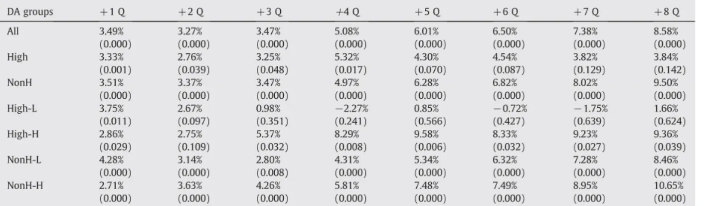
Table 5shows the two-year buy-and-hold abnormal returns (BHARs) of samplefirms. Consistent with prior studies (e.g.,Ikenberry et al., 1995), we see a turn-around in abnormal returns surrounding a buyback announcement for the overall sample. While the average prior one-year abnormal return is−14.6% (seeTable 1), the average compounded two-year post-announcement abnormal return is positive, +8.6% (p-value = 0.000). When this stock performance is conditioned by DA quintile, wefind strikingly different results. Forfirms classified in the bottom four DA quintiles (NonH), two-year post-announcement abnormal returns are positive and significantly different from zero (9.5% withp-value of 0.000). Conversely, for the highest DA quintile, the two-year abnormal return is much smaller, 3.84%, and not significantly different from zero at conventional confidence levels. Although the abnormal returns of High DAfirms are significantly positive in thefirst few quarters, significance disappears after quarter +6.

Although not reported here, each of the four DA quintiles which deﬁne the NonH group has positive drifts withp-values below 5%.

While buybackfirms overall do well, the highest DA quintile is the only group which does not show a statistically significant long- horizon drift. When this group is further divided based on stock performance in the quarter prior to buyback announcement, wefind even more striking differences. For High-Lfirms where managements seemed to be under greater pressure, their abnormal stock performance is close to zero starting in quarter +3 and continuing through quarter +8, with negative average abnormal returns in some quarters, albeit insignificant. Yet for High-Hfirms, the two-year post-announcement drift is positive and significant, 9.4% (p- value = .039). When we examine the bottom four DA quintiles in a similar fashion (i.e., NonH-L and NonH-H), we do notfind any meaningful difference in two-year abnormal return between these two groups. This result suggests that the prior returns are not closely related to post-announcement performance for the bottom four DA quintiles.

The fact that the drift, on average, for the High DA sub-group is about zero but when subdivided further on the basis of prior returns leads to distinctly separate two-year abnormal drift patterns suggests that while our approach of using accruals as a proxy for managerial intent may have merit, it is also (not surprisingly) a coarse metric. When we look at a more reﬁned measure, the results are stronger. Moreover, as we subdivide the evidence further, we also conclude that the total number of buybacks where managers may have been intending to mislead investors, while non-zero, also appears to be limited.

One might expect that if managers send misleading signals to the market, the company's stock would eventually be penalized and thus underperform the market. While plausible, one also does not expect stock prices to diverge away from their fair value. As such, this limits the price“correction”or penalty one might anticipate for mimickingﬁrms to only the reversal of the initial buyback announcement return.

Recall, that the scale of this return is only around 2%, a level of mispricing that is difﬁcult to distinguish from noise when evaluating long- Table 4

Stock option holdings and exercises of top executives.

DA quintiles Unexercised vested options

Exercised options

Year−1 Year1 Year 2 Year 2−Year−1 Year 1−Year−1 Year−1 Year 1 Year 2 Year 2−Year−1 Year 1−Year−1

All 1.26% 1.38% 1.51% 0.30%⁎⁎⁎ 0.14%⁎⁎⁎ 0.21% 0.27% 0.27% 0.06%⁎⁎⁎ 0.06%⁎⁎⁎

2763 2993 2871 2632 2763 2713 2943 2821 2582 2713

Low 1.29% 1.52% 1.71% 0.46%⁎⁎⁎ 0.25%⁎⁎⁎ 0.23% 0.28% 0.32% 0.09%⁎⁎⁎ 0.05%⁎⁎⁎

327 361 347 312 327 322 356 342 307 322

2 1.22% 1.32% 1.43% 0.23%⁎⁎⁎ 0.10%⁎⁎⁎ 0.22% 0.26% 0.26% 0.04%⁎ 0.04%⁎

674 736 705 643 674 666 728 697 635 666

3 1.09% 1.21% 1.36% 0.31%⁎⁎⁎ 0.15%⁎⁎⁎ 0.17% 0.23% 0.23% 0.07%⁎⁎⁎ 0.06%⁎⁎⁎

830 882 856 801 830 819 871 845 790 819

4 1.32% 1.42% 1.58% 0.31%⁎⁎⁎ 0.13%⁎⁎⁎ 0.23% 0.29% 0.25% 0.03%⁎ 0.06%⁎⁎⁎

652 699 660 610 652 639 686 647 597 639

High 1.70% 1.73% 1.78% 0.26%⁎⁎⁎ 0.07% 0.26% 0.33% 0.36% 0.11%⁎⁎⁎ 0.08%⁎⁎

280 315 303 266 280 267 302 290 253 267

NonH−High −0.49% −0.39% −0.29% 0.04% 0.07% −0.05% −0.07% −0.10% −0.06% −0.02%

(−3.83) (−3.46) (−2.55) (0.44) (0.94) (−1.69) (−1.75) (−2.36) (−0.63) (−0.35)

High-L 1.76% 1.81% 1.87% 0.28%⁎⁎ 0.04% 0.31% 0.40% 0.43% 0.12%⁎ 0.09%

140 157 154 136 140 131 148 145 127 131

High-H 1.64% 1.66% 1.67% 0.25%⁎⁎⁎ 0.11%⁎ 0.23% 0.30% 0.32% 0.09%⁎⁎⁎ 0.08%⁎

140 158 149 130 140 138 156 147 128 138

NonH-L 1.28% 1.40% 1.53% 0.30%⁎⁎⁎ 0.15%⁎⁎⁎ 0.24% 0.28% 0.25% 0.01% 0.03%⁎⁎

1219 1317 1251 1149 1219 1198 1296 1230 1128 1198

NonH-H 1.14% 1.28% 1.43% 0.31%⁎⁎⁎ 0.15%⁎⁎⁎ 0.17% 0.25% 0.27% 0.10%⁎⁎⁎ 0.08%⁎⁎⁎

1264 1361 1317 1217 1264 1247 1344 1300 1200 1247

NonH-L−High-L −0.49% −0.40% −0.34% 0.02% 0.10% −0.07% −0.12% −0.18% −0.11% −0.05%

(−2.91) (−2.49) (−2.05) (0.14) (0.80) (−1.42) (−1.65) (−2.39) (−0.96) (−0.37)

This table presents the unexercised vested options held by top-five executives and the options exercised by top-five executives. To standardize the option holdings and exercises, we scale them by total shares outstanding. Year−1 (Year 1) is thefiscal year before (of) repurchase announcement. The columns ofYear2−Year−1 andYear 1−Year−1 show the changes between Year 2 and Year−1 and changes between Year 1 and Year−1, respectively. Each measure is with 0.5 percentile winsorization for top–bottom observations.High-L(High-H) represents the highest DA quintile with prior one-quarter abnormal return that is below (above) the median prior one-quarter abnormal return of the highest DA quintilefirms.NonH-L(NonH-H) represents the bottom four DA quintiles with prior one-quarter abnormal return below (above) the median prior one-quarter abnormal return of thefirms in bottom four DA quintiles.NonH−HighandNonH-L−High-Ltest differences between the bottom four DA quintiles and top DA quintile and between NonH-L and High-L groups, respectively. Numbers in parentheses aret-statistics and numbers in italics are the numbers of observations.⁎⁎⁎,

⁎⁎and⁎indicate that the difference is signiﬁcantly different from zero based ont-statistics at the 1%, 5% and 10% signiﬁcance levels, respectively.