Submitted to the Electrical & Electronics Engineering Programme

IMPLEMENTATION OF IMAGE TEXTURE ANALYSIS

USING

GRAY LEVEL RUN LENGTH APPROACH

By

SITIHAJAR MOHD YAKOP

FINAL PROJECT REPORT

Submitted to the Electrical & Electronics Engineering Programme

in Partial Fulfillment of the Requirements

for the Degree

Bachelorof Engineering (Hons) (Electrical & Electronics Engineering)

Universiti Teknologi Petronas

Bandar Seri Iskandar 31750 Tronoh Perak Darul Ridzuan

©Copyright 2006 by

Siti Hajar Mohd Yakop, 2006

n

Approved:

CERTIFICATION OF APPROVAL

IMPLEMENTATION OF IMAGE TEXTURE ANALYSIS

USING

GRAY LEVEL RUN LENGTH APPROACH

by

Siti Hajar Mohd Yakop

A project dissertation submitted to the Electrical & Electronics Engineering Programme

Universiti Teknologi PETRONAS in partial fulfilment of the requirement for the

Bachelorof Engineering (Hons)

(Electrical & Electronics Engineering)

Puan Azrina Abd. Aziz Project Supervisor

UNIVERSITI TEKNOLOGI PETRONAS

TRO^OH, PERAK

June 2006

CERTIFICATION OF ORIGINALITY

This is to certify that I am responsible for the work submitted in this project, that the

original work is my own except as specified in the references and acknowledgements, and that the original work contained herein have not been undertaken or done by

unspecified sources or persons.

Siti Hajar Mohd Yakop

IV

ABSTRACT

With the dramatic increase of imaging techniques, there is a great demand for new approaches in texture analysis. This paper presents a new approach for texture analysis using statistical method and gray level run length matrix (GLRLM) approach as the second order statistics approach. The objective of this project is to develop algorithms inMATLAB and be able to implement image texture analysis by using the developed algorithms. This project is taken to apply statistical approach in image

analysis and classification. The method used is statistical method which is divided

into first order statistics and second order statistics. The scope of this project is concentrated in three parts which are algorithm development and verification, image

analysis and image classification. MATLAB software is used as the main tools in this

project to develop both the first and second order algorithms. From this project it is

learned that statistical approach is capable in discriminating images. For future

recommendations, this approach can be tested on a medical image to widen the scope

of practiced for statistical implementation in texture analysis.

ACKNOWLEDGEMENTS

Alhamdulillah, with blessings from Allah S.W.T., this project has been completed successfully according to the targeted time frame. I would like to sincerely thank University of Technology PETRONAS in particular for giving me a wonderful

opportunity to carry out this meaningful project.

My heartfelt gratitude and appreciation is extended to Puan Azrina Abd Aziz for her

spirit of education as my supervisor. I have learned so much from her and this project

would be less meaningful without her presence.

My acknowledgement would be incomplete without giving credit to all FYP

Committee, especially Electrical and Electronics Engineering Department who has equipped students with essential skills for self-learning. Its well-grounded graduate

philosophy has proven to be useful in the projects implementation.

Finally, my appreciation goes to my partner for this project, Miss Norhidayah

Jamaludin, my fellow friends and my family who have helped me in various tasks and

being a good team player as well as supplying me with undivided support in

completing this project.

VI

TABLE OF CONTENTS

LIST OF TABLES ix

LIST OF FIGURES x

LIST OF ABBREVIATIONS xi

CHAPTER 1 INTRODUCTION 1

1.1 Background of Study 1

1.2 Problem Statement 3

1.3 Objectives 3

1.4 Scope of study 4

CHAPTER 2 LITERATURE REVIEW 5

2.1 Introduction to Texture Analysis 5

2.2 Texture analysis Approach 6

2.3 Structural Method 7

2.4 Statistical Method 7

2.4.1 First Order Statistics 8

2.4.2 Second Order Statistics 10

CHAPTER 3 METHODOLOGY/PROJECT WORK 12

3.1 Project Design Stage 12

3.2 Implementation of Statistical Analysis Method 13

3.2.1 First Order Statistics 13

3.2.1.1 Algorithm Development 14

3.2.1.2 Verification 15

3.2.1.3 Data Analysis and Classification 15

3.2.2 Second Order Statistics 16

3.2.2.1 Algorithm Development 17

3.2.2.2 Verification 17

3.2.2.3 Data Analysis and Classification 17

3.3 Sample Images 17

3.3.1 Brodatz Textures 18

3.3.2 Aerial Images 18

3.3.3 Computer Graphic Images 19

3.4 Tools Identification 19

3.5 Tasks Accomplished 19

CHAPTER 4 RESULTS AND DISCUSSION 21

4.1 First Order Statistics Implementation 21

4.1.1 Algorithm Development ; 21

4.1.2 Verification 21

4.1.3 First Order Statistics by MATLAB 22

4.1.4 Data Analysis and Classification 26

4.2 Second Order Statistics Implementation 28

4.2.1 Algorithm Development 28

4.2.2 Verification 28

4.2.3 GLRLM Approach 28

4.2.4 Data Analysis and Classification 30

CHAPTER 5 CONCLUSION 32

5.1 Summary 32

5.2 Future Recommendation 32

REFERENCES 33

APPENDICES 35

Appendix A Sample of Brodatz Texture 36

Appendix B Sample of Aerial Images 37

Appendix C Sample of Computer Graphic Images 38

Appendix D Histogram Representing Each Image 39

Appendix E First Order Statistics Algorithm 40

Appendix F Second Order Statistics Algorithm 43

Appendix G First Order Algorithm Verification 45

Appendix H FOS Result for Brodatz Texture 49

Appendix I FOS Result of Computer Graphic Image 51

Appendix J FOS Result of Aerial Images 53

Appendix K Tabulated Results of Array Verification 55

Appendix M Other SOS Features 56

Appendix N Flow Diagram Of The Whole Porject Work 57

Appendix O Project Milestone 59

v n i

LIST OF TABLES

Table 1 Tabulated verification results by using array 21 Table 2 Tabulated verification results by using calculation 22 Table 3 Error percentage between calculation results and array simulation 22 Table 4 Tabulated average FOS value for each type of image 23

Table 5 Tabulated FOS range for eachtype of image 23

LIST OF FIGURES

Figure 1 Illustration of deterministic type of images [16] 2 Figure 2 Illustration of stochastic type of images [16] 2

Figure 3 The scope of study of the project 4

Figure 4 Illustration of various types of image textures [16] 5

Figure 5 Block diagram of the project stages 12

Figure 6 Block diagram of image texture analysis implementation 13 Figure 7 Block diagram of the first order statistics implementation 14

Figure 8 Captured image of MATLAB M-file Editor 15

Figure 9 Block diagram of the second order statistic implementation 16

Figure 10 Example of Brodatz textures 18

Figure 11 Example of Aerial images 18

Figure 12Example of Computer Graphic Images 19

Figure 13 Example of inputimage and its histogram 22

Figure 14 Graph representation of Mean value 24

Figure 15 Graph representation of Variance value 24

Figure 16 Graph representation of Coarseness value 24

Figure 17 Graph representation of Skewness value 25

Figure 18 Graph representation of Kurtqsis value 25

Figure 19 Graph representation of Entropy value 25

Figure 20 Graph representation of Energy value 25

Figure 21 Graph representation of Median value 26

i

Figure 22 Graph representation of Mode value 26

i

Figure 23 Skewness distribution... ; 27

Figure 24 Kurtosis representation 27

Figure 25 Array representing an image 28

Figure 26 Table of GLRLM element values of four orientations 30

x

LIST OF ABBREVIATIONS

MRI Magnetic Resonance Imaging MATLAB Mathematical Laboratory Software TIFF Tagged Image File Format

CG Computer Graphic

FOS First Order Statistics

SOS Second Order Statistics

GLRLM Gray Level Run Length Method GLRLM's Gray Level Run Length Matrices SRE Short Run Emphasis

LRE Long Run Emphasis

GLN Gray Level Distribution RLN Run Length Distribution

RP Run Percentage

CHAPTER 1 INTRODUCTION

This chapter describes four subsections which are the background of study, the problem statement, the objectives of the project and the scope of study. Background of study describes the project generally and how it narrows down to the project's implementation. The problem statement will focus on the situation of the problem and research questions which lead to the objectives of the project. Lastly, the scope of study will clarify specifically the project frame and the project work boundary to ensure the feasibility within the given time frame.

1.1 Background of Study

"MRI", which stands for "magnetic resonance imaging," is a method used in medical industry to diagnose a disease. MRI uses a powerful magnet and precisely programmed radio signals to "see" inside the body. MRI images are interpreted and analyzed by the doctors manually. In some cases, the cause or defects shown in the MRI images are overlooked. This will cause a delay in the diagnosing process.

Patients with critical issues cannot be hold up in treatment. Considering this fact, instead of using traditional diagnosing method, texture analysis approach can be implemented as an alternative for a faster diagnosing result. By texture analysis method, image can be processed in less time duration. This can help in acquiring more accurate diagnosing results by using a more efficient method. This approach can be further studied for implementation in the image processing industry [1]. Thus, the objective of this project is to be able to used image texture analysis to improve currently used technique in medical image processing industry [2].

Texture analysis approach consists of two techniques namely structural method and statistical method. Texture can be defined formally in a structural manner where texture is defined formally as a field of a set of basic patterns arranged according to

1

some placement rules. This type of texture is generated by one or more basic local patterns that are repeated in a periodic manner over some image region. This definition is most applicable to deterministic types of textures such as line arrays, checkerboards and hexagonal tilings. Otherwise, a texture can be defined in a statistic manner as a stochastic field of homogenous intensity variations. This type of image texture such as aerial photograph of the earth does not seem to possess an isolated basic pattern nor a dominant repetition frequency and instead they seem to possess some random structure. Figure 1 and Figure 2 are examples of the deterministic and stochastic types of image texture accordingly [3].

w x - x w w :•-:

V - v . v . v . v m v . %

'.V.V.'.VAV.V.VJ

Figure 1 Illustration of deterministic type of images [4].

Figure 2 Illustration of stochastic type of images [4].

For this project, statistical method is chosen instead of structural method and the gray level run length method (GLRLM) will be used to perform the second order statistics.

Statistical method is chosen because of the advantages offered by it which are first;

this type of analysis is good in 'micro textures' (small scale texture) and poor performer in 'macro textures' (large scale texture) and secondly; this method is the more common and less complicated compared to structural method. Furthermore, since structural method is rarely used, the method is not highly developed. For the second order statistic, GLRLM is used for three main reasons. The major reason for the use of the GLRLM is that the length of the runs reflects the size of the texture

elements. Furthermore, the GLRLM matrices also contain the information about the alignment of the texture. Finally, the surface slant and the surface tilt of a textured surface are also reflected in the GLRLM matrices. This shows that the GLRM matrices respond to the range and orientation of a textured surface in a direct and meaningful way [4].

Improvements can be done in various ways for image processing technology. A solution to the texture analysis problem will greatly advance the image processing and pattern recognition fields and it will also bring much benefit to many possible applications in the areas of biomedical image processing (cell analysis), industrial automation (quality control) and remote sensing (crop estimation, ecology studies,

etc.) [3].

1.2 Problem Statement

Image texture analysis has been widely used in image processing field to analyze any type of digital image to provide information on characteristics of the image. Features relating to the image properties produced by texture measures are extracted, calculated and classified. Different types of images show different texture and pixel distribution pattern in an image. These differences will then be used to classify the

properties of the image and identify the type of the image.

1.3 Objectives

For this project, the objectives to be met are as follows:

1. To design the algorithms of texture analysis by using MATLAB for both first order and second order analysis.

2. To verify the algorithms written by simulation and calculation.

3. To be able to analyze the image by usingthe algorithm developed.

4. To classify the images analyzed by statistical method.

5. To perform an effective implementation of the algorithms and enhance the existing technology in image processing field.

1.4 Scope of study

Figure 3 indicates the scope of study of the project. The main section involves four

essential procedures. Specifically, this project is focused on developing the algorithm of first order and second order statistics, verification process, implementing the algorithm and classifying the images. The algorithm is developed by using MATLAB software. In order to prove that the algorithm is accurate, verification is made by calculation and array simulation. Afterwards, the sample image is fed into the system to be simulated. The output represents the characteristics of the image fed. From the features extracted, the image is then classified according to their types.

Figure 3 The scope of study of the project.

The project is given a one year time duration to be completed. To organize the project

flow, the tasks are divided into two main categories which are:

1. Software development

i. Part I: Developing and verifying the first order statistic's algorithm by

using MATLAB.

ii. Part II: Developing and verifying the second order statistic's algorithm by using MATLAB.

2. Analyzing and classifying images.

CHAPTER 2

LITERATURE REVIEW

This chapterdescribes the analytical, critical and objectivereview of written materials on the project. It provides the background information on the research area and to identify the existing discovery about image texture analysis. This section contains all the relevant theories, hypotheses, facts and data which are relevant to the objective and the findings of the project.

2.1 Introduction to Texture Analysis

Texture is an important characteristic for the analysis of many types of images. It can be seen in all images from multispectral scanner images obtained from aircraft or satellite platforms (which the remote sensing community analyzes) to microscopic images of cell cultures or tissue samples (which the biomedical community analyzes)[5].

p r a . I'-L.

?Vr I>/*••

Figure 4 Illustration of various types of image textures [4]

Figure 4 shows various types of textures. Nature gives us so many different types of image texture which varies in many ways. Visual textures are spatially extended visual patterns of more or less accurate repetitions of some basic texture elements, called texels. Each texel usually contains several pixels. Its characteristics and placement can be periodic, quasi-periodic or random. Thus, textures may have statistical or structural properties, or both. Texture features characterize the statistical

or structural relationship between pixels (or texels), and provide measures of properties such as contrast, smoothness, coarseness, randomness, regularity, linearity, directionality, periodicity, and structural complexity [6].

In digital image, texture is depicted by spatial interrelationships or spatial arrangement of the image pixels. Visually, these spatial interrelationship or arrangements of image pixels are seen as changes in intensity patterns or grey tones.

Thus in automatic analysis, information about texture has to be derived from gray tones of the image pixels. Because of various textures available, several types of

texture analysis approach evolved [7].

2.2 Texture analysis Approach

A number of texture analysis methods have been proposed some of which are frequently referred to in the correspondence. Haralick [8] categorized the various proposals into three groups: the statistical techniques, the structural methods and the statistical-structural approaches.

Statistical methods are often based on accumulating second or higher order statistics (matrices), and using feature vectors that describe these probability distributions directly, and therefore describe the image texture only indirectly. Structural methods are based upon an assumption that textures are composed of texels (structural relationship between pixels) which are regular and repetitive. Both texels and placement rules have to be described. Structural-statistical methods characterize the texel by a feature vector and describe the probability distribution of these features statistically [6].

A major disadvantage of almost all of these approaches is that they do not have general applicability which means they cannot be applied to different classes of textures with reasonable success. For instance while the statistical techniques are generally good for micro textures (small scale texture) and are poor performers on macro textures (large scale texture), the reverse is the case for structural techniques.

Another disadvantage of some of the existing methods is the computational cost

involved, either in terms of memory requirement, computation time or

implementation complexity [6].

2.3 Structural Method

The structural approach assumes that a set of primitive units ("pattern") can be easily identified. It then defines the texture as a combination ofsuch primitives according to different placement rules. There are two major problems with this approach. First, it

is not so easy to identify the primitives unless the texture is artificial or not too

complex. Secondly, the definition that the patterns are repeated according to some pre-specified rules should allow for a random change in the replication process and

the same should apply for the patterns themselves [3].

Haralick [8] remarks that tone (primitives) and texture are not independent concepts;

when there is little variation oftonal primitives, the dominant property ofthe image is tone and when there is a wide variation of tonal primitives, the dominant property of that image is texture. Structural method is cognitive rather than a perceptual approach and it would usually rely on a prior knowledge. All taken into consideration, the structural approach is not yet widely used and therefore, this approach is not very highly developed. Hence, for this project statistical approach is chosen for the

analysis [3].

2.4 Statistical Method

The statistical ("impressionistic") approach extracts a set of parameters ("features")

from a given image. The parameters are then used as the input features for classification using the well known techniques of statistical pattern recognition. The parameters are derived over the space or frequency domain. Some of the main statistical methods are mentioned next. The gray level difference method estimates the probability density function for difference taken between picture function values.

The spatial gray level dependence method estimates the joint gray levels located at a distance "d" and an angle "a". The gray level difference and the joint gray level distributions are also known as the first and second order statistics respectively. The second order statistics are usuallytabulated as co-occurrence matrices [3].

Furthermore, the first order statistics are embedded in second order statistics as marginal density functions. Thus we cannot find two pictures with identical second order statistics and different first order statistics. Usually a reduction in the number of gray levels via histogram equalization techniques is a necessary processing step for computational efficiency. Common features extracted from above statistics are the mean, variance (spread of distribution), coarseness, skewness (tiltness of distribution) and Kurtosis (Sharpness of distribution). The gray level run length method estimates the length of identical runs, where an identical run is defined as a set of connected pixels having the same gray level [3].

The first and second order statistics are by far the most used statistical methods for texture discrimination. One problem with these methods is defining the distance "d"

and the angle "a" which would fully specify the method. Davis [9] pointed out that a statistical method relates both the partition of an image into cells and subsequently with the assignment of gray levels to the cells. The first and second order statistics as defined by Haralick [8] mainly related withthe assignment aspect.

2,4.1 First Order Statistics

First order statistic is not a great value in providing texture information but they are conceptually simple and may be used to pre-process the signal before applying second order statistics. The properties frequently used are the first four moments of the image. These are obtained from the histogram of the image [8].

Let b be a random variable representing the pixel intensity, 0 < b < L-l, where L is the number of distinct grey level; and let P(b) be the corresponding histogram of the image defined such that if N(b) is the number of pixels of intensity b in the image and M is the total number of pixels in the image then [7]:

P(b) =^ (2.1)

The first four moments are then defined as:

l.Mean m=^bP(b) (2.2)

6=0

The mean gives the average greylevel of the image.

1-1

2. Variance a2 =£(6-m)2P(&) (2.3)

The variance is of the significance in texture description. A texture with a

small variance represents one in which the image tends to be relatively

smooth. A measure of the coarseness of a texture may be defined in terms of

the variance as:

Coarseness = 1 - (2.4)

1 + cr

1 L-\

3. Skew skew= — Y(b-m)3P(b)

Skewness is a measure of the symmetry of the histogram.

1 L~l

4. Kurtosis Kur = — £ (b - m)4P(b)

& 6=0

Kurtosis indicates the flatness of the histogram.

(2.5)

(2.6)

Other first order statistics are:

5. Energy eng= £[p(*)2] (2.7)

6=0

Large values of energy correspond to homogenous regions.

z,-i

6. Entropy etp =£?(&)log[>(&)] (2.8)

Large values of entropy imply a more uniform distribution of grey levels.

*-l L-\ i

7. Median med - kwhen £ P(b) =£ ?(&) =- (2.9)

6=0 b=k 2

The median gives the value of the middle grey level.

8. Mode mod = kwhen P(k) > P(b) for 0 < b < L-1 (2.10) The mode gives the most frequently occurring grey level and is most useful when there is a single sharp maximum in the histogram.

Texture measures using the histogram only do not take the neighborhood relations between pixels into consideration. To do this, second order statistics need to be used PI

2.4,2 Second Order Statistics

In this project, the gray level run length method (GLRLM) is used for second order

statistic. This approach is based on computing the number of gray level runs of various lengths. It characterizes coarse textures as having many pixels in a constant

gray tone run and fine textures as having few pixels in a constant gray tone run. A

gray level run is actually a set of linearly adjacent picture points having the same grey level value. The length ofthe run isthe number ofpicture points within the run [10].

GLRLM is actually the probability of several connected co linear pixels so close in

gray level that they form "gray level runs". A gray level run is a set of consecutive, collinear picture points having the same gray level value. The length of the run is the

number of pixels in a run. All the features of GLRLM contain run length or gray level

and never have both of them at the same time. Stated below are some of the properties of GLRLM.

1. It does not capture the true shape aspects of texels.

2. Discard information on contrast between gray levels.

The element r' (/, j |d) of the gray level run length matrix

R{0)=[riij\e)] (2.11)

specifies the estimated number of times a picture contains a run lengthyfor gray level i in the angle 9 direction. For a given picture, a set of the gray level run length matrices is computed for runs with any given direction. However, only four gray level

run length matrices£(#),# = 0°,45°,90°,135°, are computed for each picture. From

each of these matrices, five features are computed. They are as follows:

i Na-INR „t /• j\n\

1. Short Run Emphasis Willie)) =—]T £ V^' ;

TR ,=o j-\ j

i JVG -1 NR

2. Long Run Emphasis &F2{R(o)) =—X Yufr%j\d)

TR /=0 j=i

tf«-l -|2

3. Gray Level Distribution RF3(r(o)) =—J]

?i i-o

5>'M*)

7-1

1 Mr V^g -i i2

4. Run Length Distribution RFa(r(o)) =—£ ]>/'(/,yj#)

* >=iL '=°

5. Run Percentages

lp i=Q j=l

(2.12)

(2.13)

(2.14)

(2.15)

(2.16)

where NG is the number of gray levels, and NR is the number of run length in the

matrix

Ji =S 2>'(M*)

i=0 ;=1

and TP is the number of points in the picture.

(2.17)

Each of the features is actually a distinguished primitive characteristic or attribute of an image field. After normalizing the gray level run length matrices, numerical measures are then extracted. They can be used to characterize the image texture statistically.

11

CHAPTER 3

METHODOLOGY/PROJECT WORK

Methodology of the project is the branch of philosophy that analyzes the principle and procedures of this project. This chapter outlines the project stages individually by each stage, the project flow generally, the implementation of the statistical analysis method in particular, the sample of images used in the analysis and tools which are

relevant to this project.

3.1 Project Design Stage

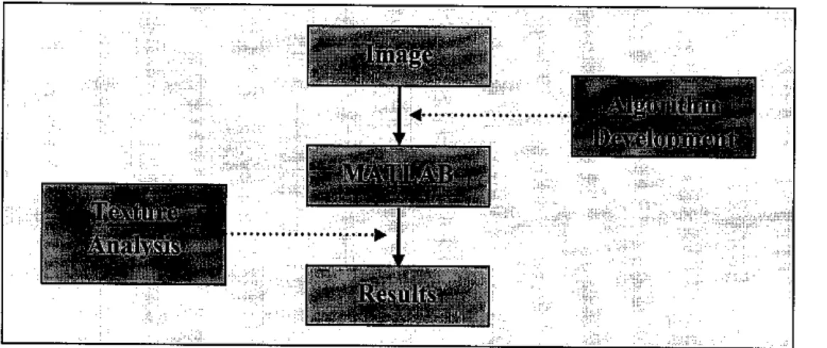
Figure 5 Block diagram of the project stages.

Figure 5 illustrates that the project stage is broken down to four sub stages which are first; research, where all data and information supporting the project scope is compiled and studied. The second stage is the development of the algorithm, where the first order and the second order statistics are developed. After being developed, all

algorithms are being verified through calculation and array simulation and lastly followed by data analysis and classification.

3.2 Implementation of Statistical Analysis Method

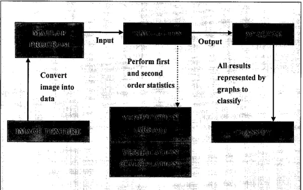
Figure 6 indicates the process flow of the statistical analysis implementation. Image will be fed into MATLAB program to be converted into a set of data which contains a set of numbers in matrix form. This data represent the histogram of the image plotted by using MATLAB program. From this histogram, properties such as total number of pixels distributed can be obtained and used in both first order and second order statistics to analyze the image. The features of each image will be extracted, analyzed and classified. Lastly before analyzing the images, the results of the first order and the secondorder statistics are represented in graphical forms to be concluded.

Convert

image into

data

Perform first and second order statistics

All results

represented by graphs to classify

Figure 6 Block diagram of image texture analysis implementation

3.2.1 First Order Statistics

In the first order statistics, the first step taken is to identify the characteristics involved to analyze the images. The characteristics are represented by a set of equations as stated in Chapter 2. These equations carry the meanings of each image.

13

From the mathematical equation, the first order algorithm is developed and verified before image analysis is applied.

NO

NO

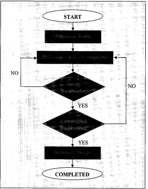
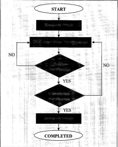
Figure 7 Blockdiagram of the first orderstatistics implementation

Figure 7 explains the flow of the first order statistics implementation process from research up until the compilation of the results.

3.2.1.1 Algorithm Development

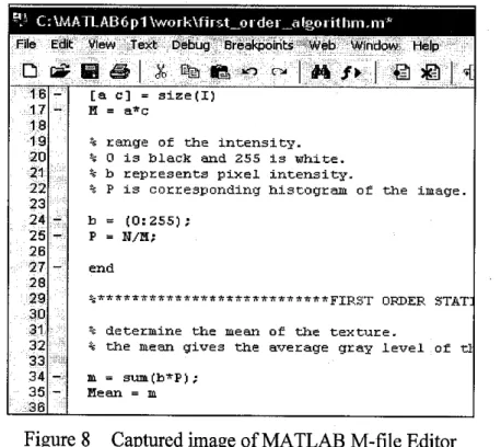
The identified problem is analyzed at this stage. Figure 7 illustrates a captured image of MATLAB M-file Editor implementation. A strong basis in MATLAB familiarization is needed to proceed from this stage. For the first order statistic, the algorithm is developed by using MATLAB M-file Editor.

^ C:\MATLAB6p1\work\first_oidei_algoiithm.m*

File Edit View Text Debug Breakpoints Web Window Help

Di*HS|*%i&««|fll/>| €l ig) | 4

16 17 18

-

[a c] = size(I)

H = a*c

19 20

% range of the intensity.

% 0 i s black and 255 i s w h i t e . 21

22 23

% b represents pixel intensity-

H P is corresponding histogram of the image.

24 25 26

;-.

b « (0:255);

P = U/H;

27 23

— e n d

29 30

%-fr****w**'ft'«ttttT'r***ttwit'W-fftt*tt*tt*£,XP^-r ORDER STAT"

31' % determine the mean of the t e x t u r e . 32

33

% the mean gives the average gray level of tl 34

35 36

-

m = sum(b*F};

Mean = m

Figure 8 Captured image of MATLAB M-file Editor

3.2.1.2 Verification

Verification of the algorithms comes after the algorithm development. During this

stage, the algorithm written by using MATLAB is verified by using two different methods. The first method is where the verification process uses different sets of array that will be fed into the algorithms and produce a set of answers. These answers of each property will be verified again theoretically, which is the second method.

Manual mathematics calculation is done to prove the array output to be correct. The results from each simulation are then tabulated and the percentage of error is

calculated.

3.2.1.3 Data Analysis and Classification

By the end of the project, the simulation results will be analyzed and a comparison study will be conducted between the results obtained by algorithm written by MATLAB and the verification results. In this last stage, the features obtained for the image is studied and analyzed. These features will tell the characteristics of each

15

image. When the classification stage is done, the projectproceeds to the second order

statistics.

3.2.2 Second Order Statistics

For the second order statistics, the method used is GLRLM approach. This method is mainly based on the run length approach, which means it uses the same statistical method as the first order to extract the textural features from a set of gray level run

length matrices (GLRLM's) ofthe images. For a given image, GLRLM's is computed

for runs with any given direction. However, only four commonly used directions

which are 0°, 45°, 90° and 135° are selected in computing the run lengths. The matrix element (i.j) specifies the number of times that the image contains a run length j as

well as having gray level i in the given direction [11].

NO

ir

'i; •

Cl_START^J^>

H H

. IHI

NO

'" :!•

X,

>

^^

'! ','

J •

~ ;

C^c^pletedJ^

'•'

Figure 9 Block diagram of the second order statistic implementation

Figure 9 exhibits how the second order statistics is being carried out. From the diagram, the first step is to develop the algorithms; then followed by algorithm verification and the last step is to analyze and to classify the image.

3.2.2.1 Algorithm Development

The algorithm is developed by computing the GLRLM's based on the equations in Chapter 2. The algorithm is written by using MATLAB software. M-file Editor provides a tool in developing the algorithm as well as to simulate the algorithm written. Since GLRLM approach involves relationships between neighboring pixels, the algorithm is needed to run in a loop to ensure all pixels are analyzed. Verification is then made to verify the results of the image analysis.

3.2.2.2 Verification

Same as the first order algorithm, the verification is done by using array as image and calculation. The percentage of error for both results is calculatedand compared.

3.2.2.3 Data Analysis and Classification

All results are tabulated and studied to classify the image. From the features extracted, the type of each image analyzed is obtained.

3.3 Sample Images

Images chosen are based on three types of images which are Brodatz textures, aerial images and computer graphics images. For this simulation, thirty different images for every image type will be fed as the input for the algorithm and all thirty images are having the same image size which is chosen to be 8 bits/pixels (black and white images or monochrome) and 512 x 512 pixels in size.

17

3.3.1 Brodatz Textures

Figure 10 Example of Brodatz textures [20]

The first type is Brodatz texture. Figure 10 shows some examples of Brodatz textures.

These images are obtained from The USC-SIPI Image Database. The USC-SIPI

image database is a collection of digitized images. It is maintained primarily to

support research in image processing, image analysis, and machine vision. The

images are in TIFF file format as supported by MATLAB. TIFF stands for 'Tagged

Image File Format', one of the most common graphic file formats for line-art and photographic images. A TIFF file always consists of pixels; it can store information at any resolution the user requests and can include color or black and white data.

Brodatz textures often are based on natures and surroundings such as grass, brick

wall, blood cells and skin of the trees.

3.3.2 Aerial Images

Figure 11 Example of Aerial images [20]

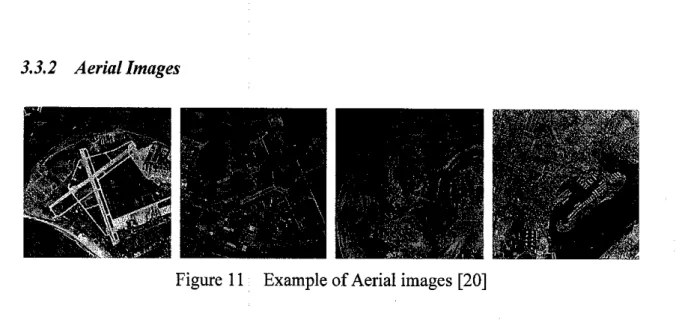
Figure 11 illustrates four samples of aerial type images. Aerial can be defined as in or belonging to the air or operating (for or by means of aircraft or elevated cables) in the air; "aerial particles"; "small aerial creatures such as butterflies"; "aerial warfare";

"aerial photography"; "aerial cable cars" [11]. Thus, aerial images are a photograph of part of earth's surface usually taken from an airplane. Thirty images of the same type

are analyzed. These images will give a range of values for each features extracted from them. Classification of images is done based on the range value obtained.

3.3.3 Computer Graphic Images

Figure 12 Example of Computer Graphic images [4]

Figure 12 illustrates four examples of computer graphic images. Computer graphic (CG) is the field of visual computing, where one utilizes computers both to generate visual images synthetically and to integrate or alter visual and spatial information sampled from the real world [12]. As other types of images, thirty sample images from computer graphic are analyzed in this project.

3.4 Tools Identification

In this project MATLAB plays a big part to get the results. Firstly, MATLAB is used to read image and convert it into a set of data and simulate the histogram which represents the image. MATLAB is also used in the verification process which goes through two different methods; first by using array simulation and secondly by mathematics calculation. Familiarization with the software helps in terms of saving time and producing good results.

Besides MATLAB, Microsoft Office Picture Manager is used to edit the image into selected size. Another tools used in preparing the images is IrfanView Software. This software is used to change any colored image into monochrome image.

3.5 Tasks Accomplished

For the first order statistics, all the tasks have been accomplished accordingly. This

19

includes the algorithm development, algorithm verification, image analysis implementation and lastly data analysis and classification. All results and data are compiled in Chapter 4 and all discussions are also provided in detail in the same chapter.

As for the second order statistic, the algorithm is developed but is having some umesolved errors which prevents the project to proceed. However, the approach implementation is discussed in this paper and the expected results are mentioned in Chapter 4. This project should run smoothly when the errors of the second order statistics algorithm are solved.

CHAPTER 4

RESULTS AND DISCUSSION

This chapter presents the findings and outcome of the project work. All the gathered data of the project work is presented and tabulated in this chapter. All findings are then discussed and analyzed through this chapter. The findings will be started with the first order statistics implementation and followed by the second order statistics implementation. Each part is sub divided into verification, results and data

classification.

4.1 First Order Statistics Implementation

4.1.1 Algorithm Development

The first order statistics algorithm is successfully developed. For further revision, the algorithm written can be referred in Appendix E.

4.1.2 Verification

As mentioned, the algorithm developed needs to be verified before the images can be analyzed by using the same algorithm for precise results. Table 1 and Table 2 show the verification done by using array simulation and mathematical calculation.

Table 1 Tabulated verification results by using array

Arrav Men h. Vanancc^iCiKirscncss, ;.. Skcjynjcss •

^utfiwif'TriV^

^{^Entropy}

1 12 604 0.9983 -0.4123 0.1711 4 0.6021

2 48 23264 1.0000 -0.2893 0.0838 16 2.4083

3 75 73630 1.0000 -0.2589 0.0671 25 3.4949

21

Table 2 Tabulated verification results by using calculation

3HHS1 '" McaiTf *1AJ$I1H|

l^a|Bjp|S^ (B^PPI^^Bx^ww^^^wl ^HK^fiftiWl^fflfiifflpS

l !.: 604 0.9983 -0.4123 0.1711 4 0.6021

2 48 23264 1.0000 -0.2893 0.0838 16 2.4083

3 75 73630 1.0000 -0.2589 0.0671 25 3.4949

Table 3 Error percentage between calculation results and array simulation

i&fB

•KSKSwREt&ilBBBMft

l 0.00

2 0.00

3 0.00

Table 3 indicates the differences between the two results are put as the percentage of error. A low percentage of error indicates a higher accuracy of the algorithm. Thus, the algorithm is verified.

4.1.3 First OrderStatistics by MATLAB

Figure 13 Example of input image and its histogram

As shown in Figure 13, each image is represented by a histogram. Histogram represents the pixel distribution in an image according to the pixel intensity. In this analysis, the range of the histogram is from zero (0) to 255. Zero represents a black and 255 represents white. This range is a default interval for monochrome image or gray scale image. Darker image means the majority of the pixels has a high intensity

or vice versa.

Table 4 Tabulated average FOS value for each type of image

Features

Types of Image

Brodatz Aerial Computer Graphic

Mean 144.287 151.767 119.7319

Variance 3351.8252 919.1 3727.5219

Coarseness 0.9992 0.9983 0.9996

Skew -0.6306 0.0857 0.0984

Kurtosis 4.9033 2.84 2.3075

Energy 0.0161 0.0125 0.0086

Entropy -2.0152 -1.9923 -2.2602

Median 148.3667 152.33 115.2667

Mode 151.0333 153.43 134.9

Table 4 indicates the tabulated average values of first order statistics for three types of image. Values of each features for each image is attached in Appendix H, Appendix I andAppendix J for reference. From the complete table, only average values of each feature are extracted to produce the FOS range for all three types of images. Image classification is performed based on the ranged formed in Table 5.

Table 5 Tabulated FOS range for each type of image

Features

Types of Image

Brodatz Aerial Computer Graphic

Mean 111.3804 to 212.8173 111.909 to 183.6457 81.2447 to 216.1798 Variance 236.0116 to 9867.8 259.4701 to 1799.4 254.5578 to 8319.5 Coarseness 0.9958 to 0.9999 0.9962 to 0.9996 0.9961 to 0.9999

Skew -2.5270 to-0.0005 -3.623 to 1.3156 -1.4653 to 1.1308

Kurtosis 1.4366 to 40.6608 1.6496 to 6.516 1.5375 to 6.9079

Energy 0.0053 to 0.1388 0.00126 to 0.0185 0.0043 to 0.0645

Entropy -2.3090 to-1.7017 -2.2312 to-1.7727 -2.3498 to-1.7377

Median 110to219 : 110 to 187 58 to 219

Mode 0 - 255 55 to 215 ^0-255

Figure 14 until Figure 22 shows the values of each features represented in graph form. The values represent each characteristics of all thirty image selected for all three types of images.

23

12000

10000 ,•*.--"•;

8000 j^jj •••"

6000 ' ^

4000 -fefcfi

2000 • :*£"

Mean

Brodatz -CG Aerial

Figure 14 Graph representation of Mean value

Variance

::•"" "W&^'^W^^^'^J^^

t" -\' No # \6 # # 4> <p

Image

Figure 15 Graph representation of Variance value

C o a r s e n e s s

1.001

0 . 9 9 9 0.998 0.997 0.996

.. •. -••••• >ft$»sKi . ,•.*••£**!«•.

•*».L-j(i;»ii-.':».T •- ..••{Sfl

0.994 - ,,»:^»!^^ -

* * 1 \° # \6 \® # ip <#>

Image

0.995 >•£., .;;. ;^j?

- Brodatz

•CG Aerial

Figure 16 Graph representation of Coarseness value

2.0000 1.0000 O.0000 -1.0000^

-2.0000 -3.0000 -4.0000 -5.0000

S k e w n e s s

Image

• Brodatz CG Aerial

Figure 17 Graph representation of Skewness value

45.0000 40.0000 35.0000 30.0000 25.0000 20.0000 15.0000 10.0000 5.0000 0.000O

K u r t o s i s

$ $> $>

Image

Figure 18 Graph representation of Kurtosis value

0.1600 0.1400 0.1200 0.1000 0.0800 0.0600 0.0400 0.0200 0.0000

Energy

•••• 3,-i--***ri

• jrx **»• IP™ -*- ** JIO. •••"• ^

* -. -•"*-.-.--j.-«*«__.**.-"-%;-VI1 -.

* -i \° <? # # # • # #

Image

Figure 19 Graph representation of Entropy value

Entropy

Imago

Figure 20 Graph representation of Energy value

25

- B radatz -CG

Aerial

- Brodatz -CG

Aerial

- B rodatz C G A e r i a l

2 5 0 2 0 0 1 5 0

1 0 0 5 0 O

M e d i a n

# $ $

Image

Figure 21 Graph representation of Median value

3 0 0 2 5 0

200 ..-.:*^

1°° m

5 0

• V-!J#*-*1

M o d e

# $ •$>

Image

Figure 22 Graph representation of Mode value

- B r o d a t z

•CG Aerial

- B r o d a t z C G A e r i a l

4.1.4 Data Analysis and Classification

When a set of values in an image has a sufficiently strong central tendency, that is a tendency to cluster around some particular value, then it may be useful to characterize the set by a few numbers that are related to its moments or features. In this project, there are nine features extracted from each image as shown in figures above.

Mean estimates the value around which central clustering of the pixel occurs according to their intensity. For a histogram distribution with a very broad 'tails', the mean may converge poorly or not at all as the number of sampled points is increased.

High mean value represents a low intensity image and low mean value indicates a high intensity image.

Variance however characterizes the width or variability of the histogram distribution.

A texture with a small variance represents one in which the image tends to be relatively smooth. An opposite features of it is represented by coarseness which

measures how coarse the image is.

The skewness characterizes the degree of symmetry of a distribution around its mean.

While mean is dimensional that is having the same units as the measured quantities of pixels, the skewness is a conventionally defined in such a way as to make it non-

dimensional. It is a pure number that characterizes only the shape of the histogram

distribution.

Pixel

frequency

Skewness

Pixel intensity

Figure 23 Skewness distribution

Figure 23 explains that a positive value of skewness signifies a distribution with an asymmetric tail extending out towards low pixel intensity (255 which represents white). When an image has zero skewness, the distribution is in fact symmetrical.

Pixel

frequency

Kurtosis

negative -v

(platykiirtic)

positive

Pixel intensity

Figure 24 Kurtosis representation

Figure 24 illustrates the shape of the histogram which is having a positive and negative value of kurtosis. The kurtosis is also a non-dimensional quantity. It measures the relative peakedness or the flatness of a distribution to a normal

27

distribution. A distribution with a positive kurtosis is termed leptokurtic; the outline of a mountain peak as an example. However, a distribution with negative kurtosis is termed platykurtic; the outline of a loaf of bread for an example. Another shape of kurtosis is termed mesokurtic which represents an in-between distribution [13].

Median gives the value of the middle gray level in the distribution and mode gives the most frequently occurring gray level in a distribution. The mode is useful primarily when there is a single sharp maximum point in the histogram.

4.2 Second Order Statistics Implementation

4.2.1 Algorithm Development

As applied to develop the first order statistics, the algorithm of second order statistics is also written by Using MATLAB. The structure of the algorithm is attached in AppendixF for reference.

4.2.2 Verification

Verification is done in mathematical approach. A set of array is selected and the

features are calculated for all four directions.

4.2.3 GLRLMApproach

Since no image has been simulated yet, an array is considered as image at this stage.

Figure 25 represents the sample array used.

.'..V!u J.i*..un i l l Hi*

Figure 25 Array representing an image

The pixels intensity located in each coordinate in the array is analyzed and arranged

back into a new table consisting run length data and gray level. The table is constructed for all four directions and represented in Figure 26. From these tables, data for g(i), r(j) and S are extracted and used as inputs for the equations as stated in Chapter 2.

Run length

1 2 3 4

Gray

level

Gray

level

Gray

level

1 2 3 4

rQ)

1 ^•* (i i)

n u ^{^} (i

II ⁱ ii i

ii ii ⁱ ii

4 4 1

P(i.j) | 0°

g(i)

3 2 3 3

S = 10

Run length

1 2 3 4 g(i)

i » i r u 2

2 n * ° " 3

3 ^ i I il 5

4 II * (I II 3

rffl 3 8 2 0 S = 13

P(U) I90°

Run length

1 2 3 4 g(i)

! n 2 ii ii~| 3

2 - - 0 ' II 4

3 2 I I II 4

4 2 2 (l li 4

rG) 7 7 1 0 S = 15

P(i.j) | 45°

29

Run length

1

1 2 3 4 g®

3 1 II (l 4

Gray ²

i •2" "n -•• o ₄

level 3 ^{(i 1 ( 1 0 7}

4

^ 2 (l II 4

r(j) 13 6 0 0 S = 19

P(i.j) 1135°

Figure 26 Table of GLRLM element values of four orientations

4.2.4 Data Analysis and Classification

From research done on the subject, it shows that the average run length values change almost linearly with the perception distance. This indicates that the run length matrix responses to the perception distance change directly. After all computational of the GLRLM's, the features can be extracted. With these features, the image can be classified in the texture classification part. The features are short run emphasis (SRE), long run emphasis (LRE), gray level distribution (GLN), run length distribution (RLN) and run percentages (RP).

Short run emphasis is used to measure the distribution of short runs. The SRE is highly dependent on the occurrence of short runs and is expected large for fine textures. Long run emphasis measures distribution of long runs. The LRE is highly dependent on the occurrence of long runs and is expected large for coarse structural textures. The gray level distribution however measures the similarity of the length of runs through out the image. The RLN is expected small if the run lengths are alike through out the image and the gray level distributions measures the similarity of gray level values through out the image. The GLN is expected small if the gray level values are alike through out the image. Lastly, the run percentage measures the homogeneity and the distribution of runs of an image in a specific direction. The RP

is the largest when the length of runs is 1 for all gray levels in specific direction.

Other extra features can be referred inAppendix M.

31

CHAPTERS CONCLUSION

This chapter highlights the summary and the most significant findings of the project.

Together with the conclusion derived from the project work, future recommendation is also described in this chapter.

5.1 Summary

The first order and the second order statistics have been successfully developed in MATLAB. Through this project, it is learned that the statistical method developed are

capable in discriminating image.

5.2 Future Recommendation

As future work, further investigation can be done on the run-length statistic for to determine the most relevant features among the five features presented in this paper.

This investigation will allow the removal of the highly correlated features, while keeping the most importantones.

A test to this approach on CT studies can be done in future for comparison and classification on medical imaging field. As a final goal, successful use of the texture

features presented in this paper to develop an automated and reliable system for

analysis and classification for medical images canbe revised and developed.

REFERENCES

[I] Final Year Project Committee, Electrical & Electronics Department, University of Technology PETRONAS, Bandar Sri Iskandar, 31750 Tronoh, Perak, Malaysia, October 2005.

[2] Robert M. Haralick. K Shanmugam and Its'hak Dinstein, "Textural Features for Image classification, IEEE Transaction on system", vol.SMC3, No.6, pp.

610-621, November 1973

[3] Harry WECHSLER, Dept. of Electrical Engineering and Computer Science, University of Wisconsin, Milwaukee, WI 53211, USA, 26 November 1979.

[4] http://artworks.avalonweb.net/gallery/gallery_main.php

[5] R. M. Pickett, "Visual analyses of texture in the detection and recognition of objects", in Picture Processing and Psychopictorics, Lipkin and Rosenfeld, Eds. New York: Academic Press, pp. 289-308,1970.

[6] Fritz Albregtsen, Department of Informatics, University of Oslo, Selected Themes from Digital Image Analysis: Statistical Texture Analysis Static or Adaptive, INF 5300, V-2004,18 February 2004.

[7] Moses Amadasun, Member IEEE, and Robert King, "Textural Features Corresponding to Textural Properties", IEEE Trans, on Systems, Man and Cybernetics, Vol. 19, No. 5, September/October 1989.

[8] Robert M. Haralick, "Statistical and Structural Approaches to Texture", IEEE vol.67, No.5, May 1979 pp.786-804.

[9] L. Davis, S. Johns and J. K. Aggarwal, "Texture analysis using generalized co-occurrence matrices", IEEE Trans. Pattern Analysis and Machine Intelligence, Vol. 1, No. 3, July 1979, pp. 251-259.

[10] M. M. Galloway, "Texture analysis using gray level run lengths", Computer Graphics Image Processing, Vol. 4, pp. 172-179, June 1975.

[II] http://www.google.com dictionary search: Define aerial.

[12] http://www.google.com dictionary search: Define computer graphic.

33

[13] Horng-Hai Loh, Jia-Guu Leu, "The Analysis of Natural Textures Using Run Length Features", IEEE Trans. On Industrial Electronics, Vol. 35, No. 2, May

1988.

[14] M. Tuceryan and A.K. Jain, "Texture Analysis", Chapter 11 in The Handbook of Pattern Recognition and Computer Vision, C.H. Chen, L.F. Pau, P. S. P.

Wang (eds) World Scientific Publishing Co., pp. 235-276,1993.

[15] L. Van Gool, P. Dewaele and A. Oosterlinck, Texture Analysis Anno 1983, Computer Vision, Graphics and Image Processing, Vol. 29, pp. 336-357,

1985.

[16] A. K. Jain and F. Farrokhnia, Unsupervised Texture Segmentation Using Gabor Filters, Pattern Recognition, Vol. 24, No. 12, pp. 1167-1186,1991.

[17] D. Blostein, N. Ahuja, Shape from texture: Integrating texture-element extraction and surface estimation, IEEE Trans. Pattern Analysis and Machine Intelligence, Vol. 11(12), pp. 1233-1251,1989.

[18] Kalle Karu, "Is there any Texture in the Image?", Dept of Computer Science, Michigan State University, East Lansing, MI 48824.

[19] Richard W. Conners, "A Theoretical Comparison of Texture Algorithms, IEEE Transactions on Pattern Analysis and Machine Intelligence", vol.PAMI- 2,No.3,May 1979

[20] http://sipi.use.edu/database.

APPENDICES

Appendix A Sample of Brodatz Texture

Appendix B Sample of Aerial Images

Appendix C Sample of Computer Graphic Images

Appendix D Histogram representing each image

Appendix E First Order Statistics Algorithm

Appendix F Second Order Statistics Algorithm

Appendix G First Order Algorithm Verification

Appendix H FOS Result for Brodatz Texture

Appendix I FOS Result of Computer Graphic Image

Appendix J FOS Result of Aerial Images

Appendix K Tabulated Results of Array Verification

Appendix M Other SOS Features

Appendix N Flow Diagram Of The Whole Porject Work

Appendix O Project Milestone

35

APPENDIX A

SAMPLE OF BRODATZ TEXTURE

Published with courtesy of http://sipi.use.edu/database/

APPENDIX B

SAMPLE OF AERIAL IMAGES

Published with courtesy of http://sipi.use.edu/database/

37

APPENDIX C

SAMPLE OF COMPUTER GRAPHIC IMAGES

Published with courtesy ofhttp://artworks.avalonweb.net/gallery/gallery_main.php

APPENDIX D

HISTOGRAM REPRESENTING EACH IMAGE

Brodatz Image

. ,.J*-V' _{*" 1 *}

Computer Graphic Image

m

"-Hi

Aerial Image

39

APPENDIX E

FIRST ORDER STATISTICS ALGORITHM

% read the input of the image.

I = imread('30.tiff);

figure, imshow(I);

% define the image in the histogram.

% intensity of the image can be determined from the histogram.

figure, imhist(I);

N = imhist(I);

% N is the number of pixels for each intensity.

% M represents the size of the image.

% find the total pixel (M) if the image.

[a c] = size(I)

M = a*c

% range of the intensity.

% 0 is black and 255 is white.

% b representspixel intensity.

% P is corresponding histogram of the image.

b = (0:255);

P = N/M;

end

o^************************* * *FTRSTORDER STATISTICS* * **************************

% determine the mean of the texture.

% the mean gives the average gray level of the image.

m = sum(b*P);

Mean = m

% determine the variance if the image.

% small variance represents smooth image.

v = sum(((b-m).A2)*P);

Variance = v

i

\

% determine,the coarseness of the image.

c = l-(l/(l+v));

i i

Coarseness = c;

% determine the skewness of the image.

%skewness represents the measure of the symmetry of the histogram.

s = (l/v.A(3/2)).* sum(((b - m).A3)*P);

Skewness = s

% determine kurtosis of the image.

% kurtosis indicates the flatness of the histogram.

k = (1/v A2).*sum(((b-m) A4)*P);

Kurtosis - k

%determine the energy.

% large value of energy coreesponds to homogenous regions.

eng = sum(P A2);

Energy = eng

% calculate the entropy.

% function 'find' is to find the indices of the probabilities non equal to zero.

% large value of entropy implya moreuniform distribution of gray levels.

f=find(P>0);

etp = sum(P(f).*IoglO(P(f)));

Entropy = etp

% calculate the median.

% median gives the value of the middle gray level.

somme = 0;

i = 0;

while(somme<=0.5) i = i+U

somme = somme+P(i);

end

Median = i-1

41

% calculate the mode.

% mode gives the most frequently occuring gray level.

d = max(P);

Mode = find(P>=d)-l

%**#**********************************£ND**************************************

APPENDIX F

SECOND ORDER STATISTICS ALGORITHM

I = [1 1 4 4 1;3 4 0 1 1;5 4 2 2 2;2 1 1 4 4;0 2 2 5 1]

[a b] = size(I) % size of input array

% declare R as 1 by 10 matrix of zeros

% declare G as 1 by 10 matrix of zeros

% x range of ROI matrix R = zeros(l,10);

G = zeros(l,10);

forx = 2:(a-l) fory = 2:(a-l)

M = (a-2)*(b-2);

S = sum(R(j=l:R);

% y range of ROI matrix

% size of ROI matrix

% total no of runs in an image P(I(x,y)+l)