Questions regarding the use of the book should be directed to the Rights and Permissions Department of INTECHOPEN LIMITED ([email protected]). The publisher assumes no responsibility for any damage or injury to persons or property resulting from the use of materials, instructions, methods, or ideas contained in the book.
Long-range interactions
Equilibrium
Quasi-stationary states
A statistical description for the quasi-steady states of the dipole-type Hamiltonian mean-field model based on a family of Vlasov solutions. A statistical description for the quasi-steady states of the dipole-type Hamiltonian mean-field model based on a family of Vlasov solutions.
O 3 by the Mean Field Theory
Introduction
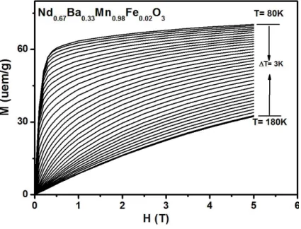
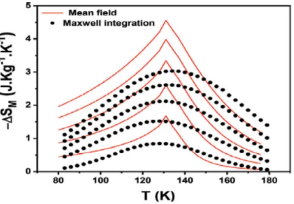
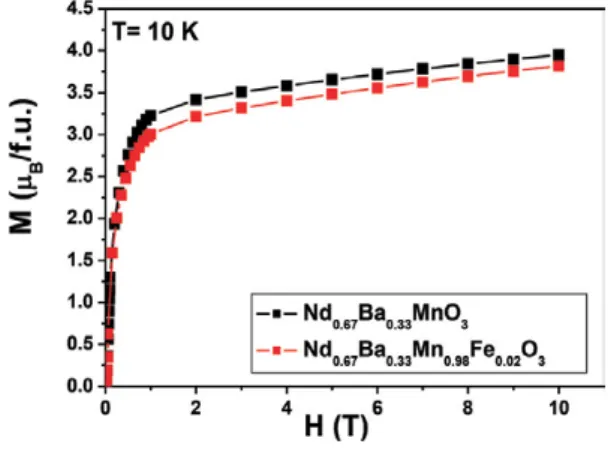
These parameters are needed to simulate magnetization isotherms, M H;ð TÞ, used for the calculation of the magnetic entropy change (�ΔSM) of Nd0.67Ba0.33Mn0.98Fe0.02O3.
Theoretical and experimental study 1 Brief overview of the experimental study
- Theoretical calculation
- Mean field theory application
This is due to the presence of the magnetic moments of Nd3þ( Xe½ �4f3Þ, which has three electrons in the 4f orbital. The Nd0.67Ba0.33Mn0.98Fe0.02O3 compound, the Mn ion located in the center of the pseudo-cubic cell from N3 has four nearby neighboring cells.
Conclusion
For a simple reason, we can consider that if this scaling method does not follow the mean field behavior, other methods must be convinced in the interpretation of the magnetic behavior of the system. The mean field theory in the study of ferromagnets and the magnetocaloric effect, thermodynamics - systems in equilibrium and non-equilibrium.
Study area
Methodology 1 Geological survey
- Geophysical study
To the east, there are outcrops of the Caracol Formation, of the Upper Cretaceous [7] forming hills protruding from the plains (Figure 3). In arid volcanic regions, one of the possibilities of locating groundwater in the enclosed aquifers is for faults. Conversely, equispaced or the vertical variation of resistivity can be studied through vertical electric soundings (VES).
In this way, we have knowledge of the change in electrical resistance in a horizontal direction. Quantitative interpretation is performed using commercial software that allows an inversion of the resistance data [22].
Results
- Air Magnetometry
- Ground Magnetometry
- Electrical methods
In the W part of the RMPF there is a "trend" of magnetic highs (red) that represents the W boundary of an area of the graben that exists with a general direction N-S and is characterized on the map by anomalies associated with magnetic lows (blue color). In the upper part, the residual magnetic field (RMF) is plotted (red); the horizontal gradient of the RMF is depicted in the lower part (blue), and at the bottom a qualitative interpretation of the percentage of probabilities of association with fracturing in the subsurface is shown. In the upper part, the residual magnetic field (RMF) is plotted (red); the horizontal gradient of the RMF is depicted in the lower part (blue), and at the bottom a qualitative interpretation of the percentage of probabilities of association with fracturing in the subsurface is shown.
In the upper part, the residual magnetic field (RMF) is shown (red); the horizontal gradient of the RMF is shown at the bottom (blue), and at the bottom the qualitative interpretation of the percentage of subsurface fracture connection probabilities is shown. Each of the VES was compared to the VES (4) of the producing well (Figures 18 and 19).
Results and conclusions
Qualitative interpretation of VES morphology showed that the producer was well connected to the KQH curve (VES 4), among the four remaining SEVs, two were from the QQH family (VES 2 and 5), one was HKQH (VES 1) and the other was HKH (VES 3). VES' were processed and interpreted with the commercial program Resix Plus, which solves the inverse problem based on Ghosh's inverse filter method [22]. Graphs of vertical electric probes (VES) 3 and 5 and comparison with VES 4, tied to a well with a yield of the order of 16 L/s.
For example, the magnetic susceptibility and resistivity of the rocks hidden beneath the surface. On the validity of using an upward continuation integral for total magnetic intensity data.
Background of diamond NV center
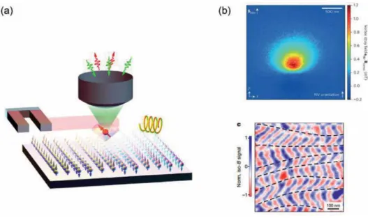
It is based on the diamond center NV (nitrogen-vacancy) which is an atomic-sized point defect in the diamond crystal providing high spatial resolution. The diamond NV center is a promising candidate to realize the goal of highly sensitive sensing with nanometer-scale resolution. The NV center of diamond is a hetero-molecular defect in a diamond crystal consisting of a substitutional nitrogen defect combined with an adjacent carbon vacancy [15, 16] (Figure 2a).
Thus, the NV center has unusually long spin coherence times even at room temperature [28] (eg T2 > 1 ms). For example, the magnetic field sensitivity of a single NV center is of the order of 1 nT= ffiffiffiffiffiffiffiffi.
Sensing mechanism
- Sensing dc magnetic field
- Sensing ac magnetic field
- Current limitations and advanced sensing protocols
The high sensitivity of the magnetic field is one of the main components of the realization of the new magnetometer presented in this chapter. DC magnetic field sensing based on Ramsey interferometry. a) Schematics of the laser and microwave pulse used for measurement. Copyright (2017) Reviews of Modern Physics. 2), the sensitivity is limited by the ESR linewidth and in principle can be as narrow as the inverse of the inhomogeneous dephasing time of the NV, T∗2.
Minimum detectable magnetic field of Bmin¼0:84�0:02μTi is obtained from the dotted line of the maximum slope. Minimum detectable magnetic field of Bmin¼0:84�0:02μTi is obtained from the dotted line of the maximum slope.
Imaging applications
- Scanning magnetometry for solid-state systems
- Wide field-of-view optics for life science
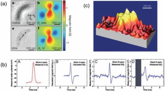
AC magnetic field detection based on CPMG measurements. a) Schematics of the CPMG pulses. coherence time compared to electron spins such as NV center. In this section, we introduce magnetic imaging techniques based on the diamond NV center. In the wide-field diamond optics experiment, ensembles of NV centers are typically used to improve field sensitivity, and biological samples are placed on a bulk diamond with NV ensembles.
Due to the capability of bio-imaging, the NV Center is gaining increasing attention in the field of neural science. The NV center is also used to investigate nuclear magnetic resonance (NMR) signal of a single protein [44] opening the possibilities of MRI at the nanometer scale [42].
Conclusions
With the TIRF configuration, the excitation laser is completely reflected from the back of the diamond at the interface between the diamond and the sample and is illuminated only on the NV ensembles. The diamond wide field of view optics successfully maps the stray field produced by a single MTB and identifies orientations of the magnetic chains of the field distribution. The premise of the BCS theory of superconductivity is a second order phonon-mediated term describing the scattering of electron pairs at the Fermi surface with momentum ki, �kien energy 2ℏωito kj, �kjwith energy 2ℏωj.
Then, in the 1950s and 1960s, an extremely complete and satisfactory theoretical picture of classical superconductors appeared in terms of the Bardeen-Cooper-Schrieffer (BCS) theory [3]. This gives the periodic part of the potential shown as the thick curves in Fig. 2 and part B, the second ionic potential.
Cooper pairs and binding
The current arises when the local volume as a whole moves due to an applied electric field. At low temperatures, phonons have no energy to break the bonds in the molecule; Electron k1 pulls/plucks at the lattice due to Coulomb's attraction, creating (emitting) a phonon and recoils to new momentum k2.
It has lower energy than the individual states in the superposition.Δbis the binding energy. Let's pause, develop this a bit in the next section and come back to our discussion.
Electron-phonon collisions
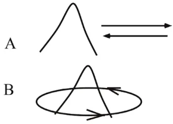
It has lower energy than the individual states in the superposition. Δb is the binding energy. Transverse phonons do not contribute to the deformation potential, as can be seen in the following. This is shown in Figure 16A. The scattering occurs through a phonon packet with width localized to the local well.
However, what is Np is really just an N number of points in the annulus around the Fermi surface that we counted earlier. The offsets are averaged by showing wave packets that are in local potential bound by phonon-mediated interaction.
BCS ground state
If there are p packet pairs on the Fermi surface, as shown in Fig. 16A, then the state arises from the superposition of the packet pairs. Representation of the Fermi sphere with the surface as a thick circle and a ring of thickness ωd (energy units) shown in dotted lines. However, of the N k-points, only N2 are inside the Fermi sphere, so we have only N2 wave packets.
The average kinetic energy of the wave packet is only the Fermi energy ϵF, since it consists of a superposition of N2 points inside and N2 points outside the Fermi sphere. If the wave packet had just been formed from a k-point inside the Fermi surface, its average energy would be ϵF�ℏω4d.
Molecular orbitals of BCS states
The average kinetic energy of the wave packet is just the Fermi energy ϵFas it consists of superposition of N2 points inside and N2 points outside the Fermi sphere. If we apply a magnetic field (say at time T) through the center of the loop, it will produce a transient electric field in the loop given by . where r is radius and ardie is area of the loop. Schematic representation of a SQUID where two superconductors S1 and S2 are separated by thin insulators.
If we turn on a magnetic field (say in time T) through the center of the loop, it will establish a transient electric field in the loop given by . Image of the schematic of a SQUID where two superconductors S1 and S2 are separated by thin insulators.
Meissner effect
A small flux through the SQUID creates a phase difference in the two superconductors (see discussion on Δk above) leading to supercurrent flow. Then, this phase change after applying the flux is from Eq. 42), δa¼δ0þeΦℏ0 across the upper insulator and δa¼δ0�eΦℏ0 along the lower insulator (see Figure 21). This accumulates charge on one side of the SQUID and leads to a potential difference between the two superconductors.
The SQUID can be thought of as a flux-to-voltage converter and can generally be used to detect any quantity that can be converted into a magnetic flux, such as electric current, voltage, position, etc. The extreme sensitivity of the SQUID is used in many different application areas, including biomagnetism, materials science, metrology, astronomy, and geophysics.
Giaever tunnelling
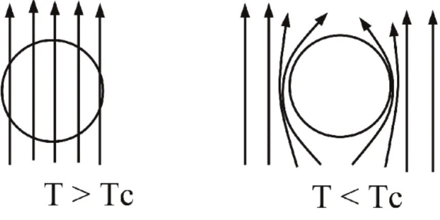
When a superconductor placed in a magnetic field is cooled below its critical Tc, we see that it expels all magnetic fields from within. German physicists Walther Meissner and Robert Ochsenfeld discovered this phenomenon in 1933 by measuring the magnetic field distribution outside superconducting tin and lead samples. A superconductor with little or no magnetic field is said to be in the Meissner state.
In the type I superconductor, if the magnetic field is above a certain threshold Hc, no expulsion occurs. Description of the Meissner effect where the magnetic field inside a superconductor is expelled when we cool it below its superconducting temperature Tc.