An accelerated, fully-coupled, parallel 3D hybrid finite-volume fluid–structure interaction scheme
A. G. Malan1,∗, O. F. Oxtoby
Advanced Computational Methods research group, Aeronautic Systems, Council for Scientific and Industrial Research, Pretoria, South Africa
Abstract
In this paper we propose a fast, parallel 3D, fully-coupled partitioned hybrid- unstructured finite volume fluid–structure-interaction (FSI) scheme. Spatial discretisation is effected via a vertex-centered finite volume method, where a hybrid nodal-elemental strain procedure is employed for the solid in the interest of accuracy. For the incompressible fluid, a split-step algorithm is presented which allows the entire fluid-solid system to be solved in a fully-implicit yet matrix-free manner. The algorithm combines a preconditioned GMRES solver for implicit integration of pressures with dual-timestepping on the momentum equations, thereby allowing strong coupling of the system to occur through the inner solver iterations. Further acceleration is provided at little additional cost by applying LU-SGS relaxation to the viscous and advective terms. The solver is parallelised for distributed-memory systems using MPI and its scaling efficiency evaluated. The developed modelling technology is evaluated by application to two 3D FSI problems. The advanced matrix-free solvers achieve reductions in overall CPU time of up to 50 times, while preserving close to linear parallel computing scaling using up to 128 CPUs for the problems considered.
Keywords: 3D fluid-structure-interaction, vertex-centered finite volume, partitioned strongly coupled, implicit, parallel
1. Introduction
Fluid–Structure Interaction (FSI) is a growing field within computational mechanics with important industrial applications, for example aeroelastic flut- ter response [1, 2, 3], design of valves in air compressors and shock absorbers [4, 5] and analysis of stresses therein, parachute dynamics [6, 7], the effect of
∗Corresponding author
Email addresses: [email protected](A. G. Malan),[email protected] (O. F. Oxtoby)
1Present address: Department of Mechanical Engineering, University of Cape Town, Pri- vate Bag X3, Rondebosch 7701, South Africa
wind on architectural structures [8, 9], and biomechanics [10, 11]. In real three- dimensional systems such as these, geometries are often complex and require the use of hybrid unstructured meshes. In addition, FSI problems are typically tran- sient or oscillatory in nature, requiring the solution of thousands of time-steps.
The result is that FSI calculations are burdened by high computational cost, which is at present a major obstacle to becoming a routinely used tool in in- dustry. However, recent progress in FSI modelling technology [4, 12, 13, 14, 15]
gives cause for optimism. In this paper we extend the multiphysics codeElemen- tal [16, 17, 18, 19, 20, 21] to three-dimensional FSI scenarios, and investigate advanced solver strategies with the aim of achieving significant improvements in parallel computational efficiency.
In order to robustly solve fluid-solid interaction problems which are phys- ically strongly coupled, it is advantageous to fully converge the entire system at each timestep. This is such that both dynamic and kinematic continuity – i.e. continuity of forces and velocities – are satisfied at the fluid/solid interface.
So-called monolithic methods ensure this by solving the entire coupled system [22, 23, 24]. Partitioned solvers, on the other hand, are more flexible in allowing independent treatment of the fluid and solid, but require more care to be taken to ensure a stable and efficient coupling procedure. Techniques which have been developed include fixed-point iteration accelerated by Aitken or gradient meth- ods [25, 26, 27, 28], coarse grid predictors [29], approximate [30, 31, 32, 33] and even exact [34, 35] Newton-type methods, and the use of reduced-order models [36]. Here we present a scheme where dual-timestepping [37, 38] is employed to effect the fully-coupled, implicit solution of the FSI system in a partitioned manner. While none of the techniques above have been employed to guarantee coupling stability, the method presented was found to be robust for the test cases presented.
In order to accomodate complex geometries, both fluid and solid governing equations are spatially discretised via a vertex-centered, edge-based finite vol- ume method [18, 39]. Edge-based methods hold the advantages of generic appli- cability to hybrid-unstructured meshes, ideal parallelisation properties and im- proved computational efficiency compared to element-based approaches [40, 41].
In the case of the solid domain, we use a hybrid between the traditional node- based finite volume method (which suffers from locking of high aspect-ratio ele- ments) and the element-based strain method [42] (which suffers from odd-even decoupling), to circumvent both of these problems [43].
In this paper fluid incompressibility is dealt with using a new artificial com- pressibility split-step method. Traditionally, incompressible solvers use pressure projection [44] techniques to derive an equation for pressure from the incom- pressibility constraint. Alternatively, artificial compressibility [45] may be used to solve for pressure in a matrix-free manner. It was however recently proposed to combine the aforementioned in order to combine the desirable properties of each [46]. Here we propose a simplified strategy where matrix-free solution is maintained through artificial compressibility, but instead of pressure projection, the consistent numerical fluxes of L¨ohneret al.[47, 48] are applied directly to the continuity equation to allow stable solution of pressure and in a manner which
is free from non-physical oscillations. As noted, the use of dual timestepping allows us to achieve a fully-coupled implicit, matrix-free solution.
The use of artificial compressibility for the fluid allows for matrix-free solu- tion and efficient parallelisation. However, since the actual speed of pressure- wave propagation is infinite in incompressible flow, pressure waves have to equalise across the entire fluid domain during every timestep, a process which can markedly slow convergence. Therefore an implicit method of solving the pressure equation, without sacrificing its matrix-free nature, can give signifi- cant returns in computation time. When considering the momentum equation, there is evidence that for transient problems, explicit timestepping can be as fast or faster than implicit matrix-free methods [48]. Through the use of dual timestepping, further performance improvement can result [49, 50] due to the increase in the allowable time-step size. In the latter work, however, the pres- sure equation is still treated in a fully explicit manner. We attempt to combine the most favourable characteristics of the cited schemes in one algorithm in or- der to furnish an efficient and robust method. As argued, dual timestepping is an attractive option for an FSI solver, and we combine this with an LU-SGS preconditioned GMRES technique, pioneered by Luoet al. [51] in the context of compressible flow, applied to the pressure equation. We further show that additional speed-ups may be achieved by applying LU-SGS relaxation to the momentum equations as suggested by L¨ohneret al. [48]. Combined with the concurrent solution of the solid via a Jacobi method, this results in a novel, fast, matrix-free, fully coupled parallel FSI solver which is suited to model com- plex strongly-coupled 3D problems. The developed technology is evaluated via application to two strongly-coupled three-dimensional problems from literature.
Metrics considered include speed-ups achieved by the advanced solver tech- niques, as well as overall parallel computing efficiency.
The outline of this paper is as follows. In Section 2 we present the govering equations for fluid and solid domains, then describe the spatial discretisation and mesh movement in Section 3. Section 4 details the numerical solvers and coupling algorithm and in Section 5, parallelisation of the code is discussed. We present numerical applications in Section 6 before concluding in Section 7.
2. Governing Equations
The physical FSI domain to be modelled consists of a Newtonian incom- pressible fluid and homogeneous isotropic elastic solid undergoing geometrically non-linear displacements. The mechanics of each is governed by the appropriate governing equations, which are described next. In this work the fluid mesh is moved in sympathy to the deforming solid and the internal nodes moved using the mesh movement algorithm described in Section 3.3.
2.1. Fluid equations
To account for movement of the mesh, described by velocity field u∗, it is necessary to describe the governing equations in an Arbitrary Lagrangian
Eulerian (ALE) reference frame. To do this we write the governing equations in weak form over an arbitrary and time-dependent volumeV(t) as
∂
∂t Z
V(t)
WdV+ Z
S(t)
Fj+Hj−Gj
njdS= Z
V(t)
QdV, (1) where
W=
W0
W1
W2
W3
=
ρ ρu1
ρu2
ρu3
, Hj =
0 pδ1j
pδ2j
pδ3j
, Gj =
0 σ1j
σ2j
σ3j
, (2)
Fj =W(uj−u∗j). (3) Here,S(t) denotes the surface of the volumeV(t) withn being a unit vector normal to S(t); Q is a vector of source terms (e.g. body forces), u denotes velocity,pis the pressure,ρis density,σ stress, andδij is the Kronecker delta.
The governing equations are closed via the relationship between stress and rate of strain:
σij =µ ∂ui
∂xj
+∂uj
∂xi
, (4)
whereµis the dynamic viscosity andxi are the fixed (Eulerian) co-ordinates.
2.2. Solid Equations
To account for large deformations without accumulating strain errors due to repeated oscillations, the solid equations are formulated in a total Lagrangian formulation, i.e. in the undeformed reference frame. In this coordinate system the momentum equations are written in weak form as
∂
∂t Z
V0
ρ0vidV= Z
S0
PijnjdS+ Z
V0
QidV, (5)
wherevis the solid velocity,Pis the first Piola-Kirchoff stress tensor,V0denotes a volume in the material coordinate system andS0its surface, withnbeing its outward pointing unit normal vector. Further, ρ0 is the solid density in its undeformed state andQ, again, a vector of source terms.
We use the St. Venant–Kirchoff model to account for finite strains. In this model, the Green-Lagrange strain tensorEis used, with components
Eij= 1 2
∂wi
∂Xj
+∂wj
∂Xi
+∂wk
∂Xi
∂wk
∂Xj
(6) wherew is the total displacement of the solid from equilibrium locationX, so that x = X+w. The second Piola-Kirchoff stress tensor S is related to the strain tensor by
Sij= 2G(Eij−13Ekkδij) +KEkkδij (7)
m
n
ϒmn
S1,1mn
S1,2mn
S2,1mn
S2,2mn
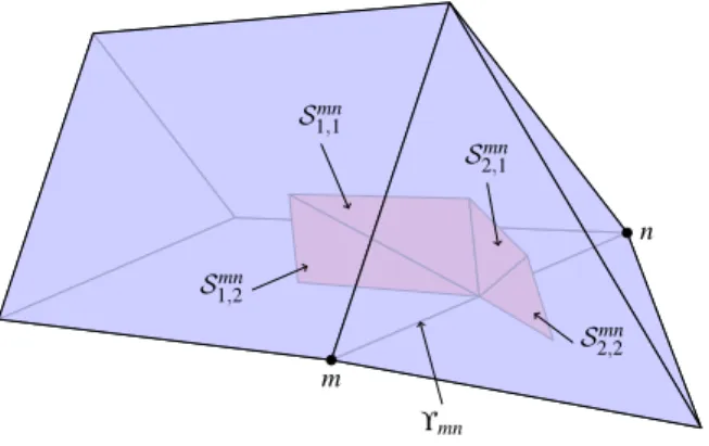
Figure 1: Schematic diagram of the construction of the median dual-mesh on hybrid grids.
Here, Υmndepicts the edge connecting nodesmandn. Shaded is the dual-cell face between nodes m and n. This is composed of triangular surfaces Sklmn which are constructed by connecting edge centers, face centroids and element centroids as described in the text.
where G is the shear modulus and K the bulk modulus (summation over k implied). Finally, we convert from the second to the first Piola-Kirchoff stress tensor,P, with
Pij=FikSkj, whereFik =δik+ ∂wi
∂Xk
. (8)
To close the system of equations, the solid velocity v and displacement w are related in the obvious way:
Dwj
Dt =vj. (9)
whereD/Dtdenotes the derivative with respect to a fixed point in the reference (initial) configuration.
3. Spatial Discretisation
3.1. Hybrid-Unstructured Discretisation
In this work, we use a vertex-centred edge-based finite volume algorithm for the purposes of spatial discretisation, where a compact stencil method is employed for all Laplacian terms in the interests of both stability and accuracy [18, 39], for both fluid and solid domains. The method allows natural generic mesh applicability, second-order accuracy without odd-even decoupling [18], and computational efficiency which is factors greater than element based approaches [40]. The edge-based method is also particularly well suited to computation on parallel hardware architectures due to the constant computational cost per edge.
Considering the fluid ALE governing equations (1), all surface integrals are accordingly calculated in an edge-wise manner. For this purpose, bounding surface information is similarly stored per edge and termed edge-coefficients.
The latter for a given internal edge Υmn connecting nodesmandn(see Fig. 1, is defined as a function of time as
Cmn(t) = X
k∈Emn
h
nmnk,1(t)Sk,1mn(t) +nmnk,2(t)Sk,2mn(t)i
(10) whereEmnis the set of all elementskcontaining edge Υmn,Sklmn is the area of the triangle connecting the centre of edge Υmn with the centroid of elementk and the centroid of one of its two faces which is also incident on Υmn, l= 1,2.
Further, nmnkl are the associated unit vectors normal to these triangles and oriented from nodem to node n. The discrete form of the surface integral in Eq. (1), computed for the volume surrounding the nodem, now follows as
Z
Sm(t)
Fj+Hj−Gj njdS ≈ X
Υmn∩ Vm(t)
n
Fjmn+Hjmn−Gjmno
Cmnj (11)
where all•mn quantities denote face values. In the case of the fluid, Gjmn = h
Gjmn
tang +Gjmn norm
i [18], where Gj
tang is calculated by employing di- rectional derivatives andGj
norm is approximated by employing the standard finite volume first-order derivative terms.
When considering the solid governing equations (5), the above method of discretising the stress term would enforce continuous gradients at nodes and element boundaries and therefore suffers from stiffness problems on stretched elements [43]. To remedy this we use the hybrid nodal/elemental strain tech- nique [43]. In this method, components of strainEij withi =j are obtained as per the above. However, the components with i 6= j are evaluated at the element centre and averaged with the neighbouring element’s value to obtain the value at the edge centre.
3.2. Geometric Conservation
In order for the fluid solution to be as transparent as possible to the move- ment of the mesh, an identity known as the Geometric Conservation Law (GCL) should be obeyed [52, 53, 54]. It asserts that the momentum flux into a cell due to the motion of the faces should be consistent with the change in momentum of the cell due to its changing volume. That is, the discretised version of
∂
∂t Z
V(t)
dV = Z
S(t)
u∗jnjdS. (12)
should hold exactly, which implies that constant spatial fields will be unaffected by arbitrary mesh deformations. The GCL can therefore be said to impose a specific relationship between mesh deformation and the mesh-velocity field. We could discretise the equation above at nodemas
Vmt+∆t−Vmt
∆t = X
Υmn∩Vm(t)
δVmnt
∆t , (13)
whereV is the volume of dual-cellV,δVmnt is the volume swept out by the face lying between nodesmandnbetween time-stepstandt+ ∆t. Then, the GCL will hold. Alternatively, to second order accuracy [54]
3Vmt+∆t−4Vmt +Vmt−∆t
2∆t = X
Υmn∩Vm(t)
3δVmnt −δVmnt−∆t
2∆t . (14)
Thus, in order for our discretisation to be consistent with the GCL, the mesh ve- locity fluxu∗jCmnj in the discretisation of (1) is set equal to (3δVmnt −δVmnt−∆t)/2∆t.
3.3. Dynamic Mesh Movement
For the purposes of mesh movement, we employ an interpolation procedure [55] which, while offering no guarantees about element quality, has no significant computational cost and is well suited to parallel computing. This approach en- tails redistributing internal fluid nodes via the following interpolation function:
∆x=r∆x1+ (1−r)∆x2,
where ∆x1and ∆x2respectively denote the displacement of the closest internal and external boundary nodes from their initial locations, and r, which varies between zero and one, is computed as
r= Dp2
Dp1+Dp2 withp= 3/2. (15) Here,D1andD2are the distances to the identified internal and external bound- ary points in the undeformed configuration. Since the values ofrare calculated only once at the beginning of the entire analysis, the parallel computational overhead of the mesh movement function is negligible; furthermore, cumulative deterioration of element quality during repeated oscillations does not occur as the mesh always returns to its initial configuration. While this method has been found to perform well for many problems which include non-linear motion (such as rotations), it is somewhat sensitive to the magnitude of motion as mesh quality is not explicitly enforced.
4. Temporal Discretisation and Solution Procedure
The solution procedure must allow for fast, parallel, fully coupled solution of all descritised equations while allowing independence in terms of discretisation and solution strategy employed for the fluid and solid domains. We therefore advocate a strongly coupled, partitioned, matrix-free iterative solution process where fluid-solid-interface nodes communicate velocities and tractions at each iteration. The resulting proposed solution procedure is detailed below.
4.1. Temporal Discretisation
For the purpose of transient calculations, a dual-time-stepping temporal dis- cretisation [16] is employed such that second-order temporal accuracy is achieved while ensuring that all equations are iteratively solved simultaneously in anim- plicit fashion. This results in a strongly coupled solution. The real-time tempo- ral term is accordingly discretised to second-order and added as a source term to the right-hand-side of the discretised fluid momentum equation as
QiV
τ=−3Wiτ+∆τVτ−4WitVt+Wit−∆tVt−∆t
2∆t fori= 1,2,3 (16)
where ∆tdenotes the real-time-step size, the tsuperscript is the previous (ex- isting) real time-step andτ denotes the latest known solution to the time-step being solved for viz.t+ ∆t.
For the solid equation, a similar source term is added to the right-hand side of the discretised version of Eq. (5), namely
QτiV0=−ρ0
3vτ+∆τi −4vit+vti−∆t
2∆t V0 (17)
and also to the discrete form of Eq. (9), to give Dwi
Dt =vi−3wτ+∆τi −4wti+wit−∆t
2∆t (18)
where the nomenclature is as defined previously.
4.2. Solution Procedure: Fluid
The solution of the incompressible fluid equations (2) presents two numer- ical difficulties. Firstly, the spatial discretisation of the convective terms via central differencing results in destabilising odd-even decoupling, and secondly, the pressure field must evolve such that the incompressible continuity equation
∇ ·u = 0 is satisfied. Since this equation does not involve pressure, solving for it in a matrix-free manner is not straightforward. We use a new artificial compressibility split-step algorithm stabilised with consistent numerical fluxes [55] (CNF-AC method) to overcome this difficulty, as described below.
For incompressible flow it is usually advocated that the pressures are solved implicitly [48] while advective (convective) terms are explicitly integrated [46, 48]. This is as the advective timescales are those of interest, whereas pressure waves propagate instantaneously. L¨ohneret al.[48] have undertaken a thorough investigation into various explicit and implicit integration strategies, with the fastest solution times for transient problems achieved using explicit integration of the advective terms. However, for strongly-coupled FSI systems, the use of an implicit fluid solution methodology allows for strongly coupled concurrent partitioned solution of both fluid and solid domains. We therefore advocate such an approach for this work.
Dual-timesteping has long been used to achieve second-order accurate tem- poral solutions without introducing the extra computational cost of a more traditional implicit solver [16, 18, 37, 38, 49]. In the context of FSI, it con- fers the additional advantage of allowing the coupled system to be implicitly solved with the sub-iteration process serving the purpose of effecting numerical strong coupling between fluid and solid. We therefore propose the use of dual- timestepping for the momentum equations combined with implicit integration of pressures.
We now describe the split-step incompressible flow algorithm. The CNF-AC scheme addresses the continuity equation directly by adding artificial compress- ibility and fourth-order stabilisation terms as follows:
1 c2τ
pτ+∆τ2−pτ
∆τ2
Vτ=− Z
S(t)
ρuk
τ+∆τ
ℓ (pR−pL)nk
τ+α∆τ2
nkdS (19) whereαcontrols the level of implicitness and ∆τ2is the iterative or pseudo-time- step size (solution involves driving the right-hand-side of the equation to zero).
Further,pRdenotes the pressure extrapolated from the node outside the control volume (denotednbelow),pLdenotes the pressure extrapolated from the node inside it (denotedm) andℓis the length of the edge connecting nodesmandn.
In the context of upwinding the aforementioned typically refer to the left and right states respectively. This stabilisation term is essentially the same as the
‘consistent numerical flux’ of L¨ohneret al.[47, 48]. Using constant interpolation (i.e. the nodal values forpRandpL) yields an effective second-order (Laplacian) stabilisation term, whereas an effective fourth-order stabilisation term results from the third-order accurate linear interpolation used in the MUSCL scheme [56]:
pL=pm+1 2
(1−κ)∇p|m·ℓ+κ(pn−pm)
, κ= 1/3. (20) Here,ℓis the vector from nodemto node n.
In the interest of computational efficiency, we use the implicit formulation (α= 1) to approximate the interpolated pressures, and in such a way as to use only nearest-neighbour values of the increment ∆p≡pτ+∆τ2−pτ being solved for:
(pR−pL)τ+∆τ2 ≈(pR−pL)τ+ (∆pn−∆pm). (21) Via numerical experimentation it is found that the computational cost of addi- tional iterations due to the inexact Jacobian is more than offset by the saving due to the greater sparsity of the Jacobian.
Having solved (19) forpτ+∆τ2, a momentum iteration follows as Wiτ+∆τ−Wiτ
∆τ Vτ=−
Z
S(t)
(Fij−Gji)njdS
τ+β∆τ
− Z
S(t)
HijnjdS
τ+∆τ2
+QiV|τ
≡Ri(W), (22) whereβis set to 1 for the implicit treatment of velocity terms and zero otherwise.
The rationale for the implicit treatment of velocities is as follows. There are two pseudo-time-step size restrictions on ∆τ in Eq. (22): the viscous timestep due to the diffusive terms inGand the convective timestep due toF. The former is often more restrictive than the latter, scaling with the square of mesh spacing rather than the mesh spacing itself. Moreover, the convective timescales are gen- erally those of interest in transient problems. This means that it is worthwhile to solve the viscous terms implicitly (provided a computationally efficient solver is used) whereas increasing the convective timestep size dramatically would result in a loss of temporal accuracy. The latter would in addition be far more com- putationally intensive as cross-coupling between all governing equations would have to be accounted for. However, to facilitate modest extensions of the allow- able convective pseudo-timestep size, convective velocity components which are not cross coupled are included in the Jacobian. This results in a nett reduction in computational cost (as will be reported on below). Thus, the convective and viscous velocity terms in Eq. (22) are treated as follows:
Fij|τ+β∆τ≈Wi|τ+β∆τ(uj|τ+δijβ∆τ−u∗j|τ) (23) and
Gji|τ+β∆τ ≈µ ∂ui
∂xj
τ+β∆τ
+∂uj
∂xi
τ+βδij∆τ
(24) fori, j = 1,2,3. Note that the second term above does not contribute to the governing equations in the case of constant µ due to the continuity equation and thus the cross-derivative terms may be treated explicitly.
Finally, the fluid mesh velocity u∗ is calculated via second-order backward difference as per Eq. (17).
4.2.1. Preconditioned GMRES Routine
As mentioned, we wish to solve Eqs (19) and (22) implicitly in order to over- come the time-step-size restrictions on ∆τ2and on ∆τto which explicit methods are subject. However, in order to scale efficiently to very large problems, the procedures must be matrix-free. Different approaches are required to efficiently solve the pressure equation (19) and the momentum equations (22), since in the former case the pseudo-time-step size should be increased as much as possible, while in the latter it remains restricted by the convective limit. Thus, it is more efficient to solve the momentum equations with more iterations of a computa- tionally less intensive solver, compared to the pressure equations, which we now consider first.
A popular approximate matrix solver is the Generalised Minimum Residual (GMRES) method of Saad and Schultz [57], which finds an optimum solution within a reduced subspace spanned by the so-called Krylov vectors. The choice of the preconditioner to be applied to the GMRES Krylov-subspace vectors is of utmost importance. It must ensure a good condition number while, im- portantly, preserving the matrix-free nature of the solution scheme and being computationally efficient. Luo et al. [51] were the first to employ LU-SGS [58, 59, 60] for this purpose. As compared to its main competitor, Incomplete
Lower-Upper decomposition (ILU), it does not require the storage of any part of the preconditioning matrix. Furthermore, it has been applied with success to the nonlinear heat conduction equation [20], showing orders of magnitude performance improvement over Jacobi iterations and even over both GMRES and LU-SGS in isolation. As the pressure equations have a diffusive character similar to the heat equation, a similar methodology was adopted for this work.
The discrete form of Eq. (19) can be written in the form
A∆p=Res (25)
where ∆p=pτ+∆τ2−pτ and Resis the residual vector. The lengths of the vectors ∆pand Resare equal to the number of nodes N, andA is a sparse coefficient matrix. An outline of the LU-SGS preconditioned, restarted GMRES procedure follows.
At each iteration the change in the primitive variable vectorpis calculated from ∆p = vlal, l = 1. . . L. Here L denotes the number of preconditioned Krylov-space vectorsvl, and the coefficients al are calculated such that they minimise the residualResfor a given set of Krylov-space vectors (the expression from which al is calculated follows below). The latter are calculated via the following GMRES procedure, which is invoked iteratively for a pre-specified number of GMRES iterations.
1. Initialise ∆p0=0.
2. Starting Krylov-subspace vector:
v1=
P−1(Res−A∆p0) P−1(Res−A∆p0)
−1 (26)
where P−1 denotes the preconditioning matrix, orP−1 ≈A−1, and | · | denotes the Euclidian norm.
3. Forl= 1,2, . . . , L−1, compute Gramm-Schmidt orthogonalisation:
wl+1=P−1Avl−
l
X
k=1
hklvk, hkl =vk·P−1Avl (27)
vl+1= wl+1
|wl+1| (28)
4. The change in pis now calculated from the expression given previously, namely
∆p= ∆p0+vlal (29)
whereal are calculated such that the residual is minimised:
Avk
· Avl
al= Avk
· Res−A∆p0
(30) 5. Restart from Step 2 using ∆p0= ∆puntil a pre-set number of iterations
complete.
We now outline the preconditioning procedure. The generic vectorω is pre- conditioned by the LU-SGS procedure by performing two computational sweeps over the mesh:
• Sweep 1: Calculateω∗ from (D+L)ω∗=ω, and
• Sweep 2: Calculateωp from (D+U)ωp=Dω∗,
where L, D and U are the strict lower, diagonal and upper parts of A. Further, ω∗ and ωp respectively denote the intermediary and preconditioned versions ofω. Note that this procedure may be implemented in a completely matrix-free form.
As mentioned, a fixed number of GMRES iterations (restarts) are used rather than running the GMRES procedure to convergence. (Recall that the GMRES method runs inside the pseudo-time iteration sequence detailed in Section 4.2, which must itself be iterated in order to reach pseudo-steady state.) For the purposes of this work it was found that efficient convergence of the overall scheme is attained with three GMRES iterations (i.e. two restarts). This is because the residual is rapidly reduced at first, with diminishing returns for further restarts.
For fastest convergence of the pseudo-timestep iterations, ∆τ2 should be made as large as possible. On the other hand, if it is made too large the performence of GMRES degrades as the A matrix loses diagonal dominance.
For the purpose of this work, ∆τ2= 105∆τ was employed.
Turning now to the implicit solution of velocity in the momentum equations (22), as mentioned, a computationally cheap solver is necessary in order to effect an overall speedup due to the convective timestep size restriction. For the same reason, however, the Jacobian remains diagonally dominant and so it is found that a single LU-SGS sweep per pseudotime iteration – computationally no more expensive than two Jacobi iterations – is sufficient to remove the viscous timestep restriction altogether [61].
The procedure is as follows. Similar to Eq. (25), the discretised form of Eqs (22) can be written in the form
Ai∆ui =Resi fori= 1,2,3, (31) where ∆ui = uτ+∆τi −uτi and Resi are the residual vectors. The LU-SGS procedure outlined above is then applied withω =ui, with ui then replaced by the calculated ωp. The speed-up in solution gained via the above will be assessed in Section 6.1.1.
4.3. Solution Method: Solid
For the majority of FSI problems, the solid domain contains far fewer equa- tions to solve as compared to the fluid. As such, a simple Jacobi iterative proce- dure was selected for this work, which involves the pseudo-temporal discretisa- tion of Eqs (5) and (18). Traction boundary conditions are realised numerically
by excluding external boundaries from the surface integral in (5) and adding in surface integrals of the applied tractionsτ. Thus, the equation becomes
∂
∂t Z
V0
ρ0vidV= Z
S0internal
PijnjdS+ Z
Sboundary
τidS+ Z
V0
QidV ≡Ri(w), (32) For pseudo-temporal discretisation a single-step procedure proposed in [62]
was used:
wiτ+∆τ=wτi + ∆τh
viτ−3wτi−4w2∆tti+wt−i ∆t +12∆τ Ri(wτ)/(ρτ+∆τ0 V0τ+∆τ)i vτ+∆τi =vτi + ∆τ Ri(wτ)/(ρτ+∆τ0 V0τ+∆τ)
(33) whereV0 is the volume of dual-cellV0in the undeformed configuration and wτ denotes a projected displacement which is calculated as
wiτ =wτi + ∆τ viτ (34)
where the nomenclature is as previously defined.
4.4. Pseudo-timestep Calculations
The pseudo-timestep local to each computational cell is to be determined in the interest of a stable solution process. For this purpose, the following expression is employed:
∆τ = CFL
|ui−u∗i|+cunified
∆xi
+κ(1−β) 2µ ρ∆x2i
−1
(35) where CFL denotes the Courant-Friedrichs-Lewy number, ∆xi is the effective mesh spacing in direction i and κ is equal to 1 in the fluid domain and 0 in the solid domain. Note that if the velocity terms are being treated implicitly (β = 1), the viscous time-step size restriction falls away. Further,
cunified=κcτ+ (1−κ)p
K/ρ0+p η/ρ0
. (36) 4.5. Solution Procedure
To achieve simultaneous solution of the discretised fluid-solid equations in a manner which effects strong coupling, the following solution sequence is em- ployed in an iterative fashion:
1. The fluid and solid discrete equations are solved concurrently via (19)–(22) and (32). Due to the accelleration of the fluid solver with GMRES, con- vergence of the fluid domain is typically faster than the solid. Therefore, in order to achieve fast convergence of the coupled system, an adjustable number of iterations of Eq. (32) may be performed for every iteration of the fluid equations.
2. At the interface, the calculated fluid traction is applied to the solid bound- ary and the solid velocities to the fluid boundary. That is, the following equations for traction and velocity at the boundary are prescribed:
τj =pnj−σijni
u=v (37)
wherenis the normal unit vector pointing outward from the fluid domain.
3. The mesh is only moved if a solid mesh boundary node displacement exceeds 30% of the attached dual-cell size or the residual of the fluid or solid mesh has been reduced by three orders of magnitude (a real- time-step is considered converged when the residual of all fluid and solid equations have dropped by at least 4 orders of magnitude); hence, the mesh is always moved at least once per timestep, and more if the residual is too large or there is significant displacement of the interface nodes during the convergence process. A mesh move involves redistribution of fluid nodes, followed by pre-processing of the mesh. The latter involves computation of edge-coefficients and finite volumes.
4. The residuals are now calculated for all equations, and if larger than the convergence tolerance steps 1–3 are repeated.
5. If the residuals are below the convergence tolerance, the real-timestep is terminated, and the next time-step entered by proceeding to step 1.
As far as fluid–structure interaction is concerned, the method above repre- sents a block-Jacobi method, which suffers from slow convergence compared to block-Gauss-Seidel or block-Newton methods. However, in the current frame- work the coupling iterations are the same as the dual-timestepping pseudo- timesteps which are numerous (typically on the order of 100 per timestep), and so this does not represent a significant performance penalty. However, in order to ensure robustness, a more sophisticated coupling method (listed in Section 1;
see [35] for an overview) should be incorporated. This is because block-Jacobi and block-Gauss–Seidel methods are known to suffer from instabilities due to the
‘added mass effect’ [63, 64, 65], which are most severe when fluid and structure have comparable densities.
5. Parallelisation
Because of the fully matrix-free nature of the numerical method at solver sub-iteration level, the mesh can be decomposed into separate subdomains for parallel operation. Firstly, in composing the right-hand side, all loops are over edges, with the operation count for each edge being very nearly identical. Sec- ondly, in performing the various sparse-matrix–vector dot products that make up the preconditioned GMRES algorithm, there is one dot product pernode;
however, the number of nonzero entries in the corresponding row of the Jaco- bian matrix is equal to the number of edges surrounding the node, plus one.
Therefore, to balance the operation count for efficient parallelisation of not only
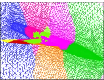
Figure 2: Example of domain decomposition.
the right-hand side calculation but also the LU-SGS/GMRES routine, the num- ber of edges in each domain was balanced. This was done by weighting each node with an integer equal to the number of edges which connect to it, followed by applying the METIS library [66] to its connectivity graph. For interdomain communication, a system of “ghost nodes” is used in this work, with one layer of overlapping nodes at domain boundaries, where ‘slave’ nodes are updated with the values from corresponding ‘master’ nodes in the neighbouring domain.
For efficiency, data transfer is consolidated into the largest possible packets and communicated using MPI. An example of the decomposition into subdomains is shown in Fig. 2, where individual domains are distinguished by colour.
The GMRES routine consists of sparse-matrix–vector products and dot prod- ucts which are suited to parallel computing. However, the LU-SGS precondi- tioning steps are formally serial in nature. These involve sweeps across the mesh, with each subsequent nodal value calculated from the newly updated val- ues of the preceding ones. While this process may be efficiently vectorised on shared-memory architectures [67], on distributed-memory machines excessive communication would be required during each sweep over the mesh, severely impairing performance. In this work we have elected to perform the LU-SGS preconditioning only within each parallel subdomain, thereby eliminating the need for communication altogether. Being merely a preconditioning step, this has no influence on the solution accuracy; neither was it found to impair stabil- ity. What does suffer somewhat is the speed of convergence, since information does not propagate across the entire mesh at each iteration to the same extent as the serial implementation. However, as demonstrated below, this effect was found to diminish as the number of parallel domains increases. When using LU-SGS for implicit relaxation of the velocities in the momentum equations,
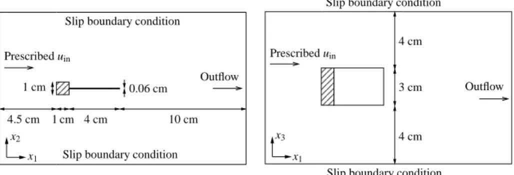
Outflow Slip boundary condition
Slip boundary condition Prescribed uin
1 cm
4 cm 10 cm
1 cm
0.06 cm 4.5 cm
x1
x2
3 cm 4 cm
4 cm Prescribed uin
Slip boundary condition Slip boundary condition
Outflow
x3
x1
Figure 3: Block with flexible tail: geometry and boundary conditions. Top view (left) and side view (right).
similar arguments apply.
6. Application and Evaluation
6.1. Block with flapping plate
The first FSI problem we consider comprises a block connected to a flexi- ble plate in cross-flow, as proposed by von Scheven and Ramm [29] and also considered by Kassiotiset al. [68] As shown in Fig. 3, it is a three-dimensional version of the popular block with flexible tail used to test 2D FSI algorithms [12, 22, 34, 42, 69].
The material properties are as follows: Incompressible fluid density is 1.18× 10⁻³ g cm−3 and viscosity µ = 1.82×10⁻⁴ g cm−1 s−1. For the plate, two different material properties have been used. We shall refer to these as the
‘stiff’ and ‘flexible’ plate respectively. In the first place, to reproduce the case considered by other researchers [29, 68], we use a densityρs= 2.0 g cm−3, and a Young’s modulusE= 2.0×10⁶g cm−1s−2. These are also the same material properties considered in the 2D analyses referenced above. Secondly, for the
‘flexible’ plate we reduce both the density and elastic modulus by a factor of 20, i.e.ρs= 0.1 g cm−3andE= 1×10⁵g cm−1s−2. This is to decrease the stiffness of the plate without affecting its characteristic frequencies, thereby increasing the three-dimensionality of the response. In both cases we use a Poisson’s ratio ν= 0.35.
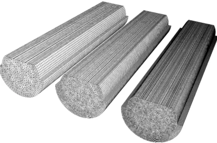
Two meshes of different densities were employed (Fig. 4) in order to assess the mesh-sensitivity of the solution. The coarse mesh consists of circa 480 000 fluid cells and 8 000 solid cells (with 6 elements through the plate thickness).
For the fine mesh the spacing was reduced by a factor of 1.5 in each direction, resulting in 1 580 000 fluid cells and 27 000 solid cells. As pointed out previously, multiple solid sub-iterations are run for every fluid mesh iteration. For the problem considered here, 30 solid sub-iterations for the coarse mesh and 50 sub-iterations for the fine mesh were found to result in similar fluid and solid drop in residual (measured between fluid-solid-boundary communication). The
Figure 4: Meshes used for block with flexible plate. Coarse mesh [(a) and (b)] and fine mesh (c).
analysis was run on a Sun Microsystems Constellation cluster with 8-core Intel Nehalem 2.9 GHz processors and Infiniband interconnects at the Centre for High Performance Computing (CHPC), Cape Town. On the course mesh, the 7 500 timesteps completed in 6 days using 23 parallel fluid subdomains and 7 solid subdomains. The fine mesh analysis took 11 days with 64 fluid and 32 solid subdomains.
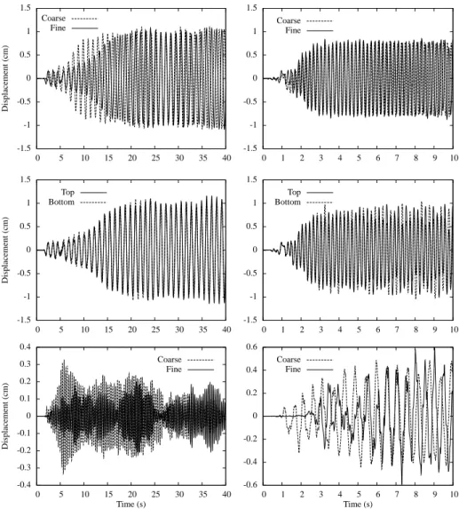
For the first analysis, with the stiffer plate, the inflow velocity was linearly ramped up to its final value of 100 cm s−1within the first 2 s of the analysis as per [29]. The time-step size was chosen as ∆t = 0.004 s. The calculated time- history of horizontal displacement of the top and bottom corners is depicted in the left panels of Fig. 5. Although there is a significant difference in the rate of growth between the coarse and fine meshes, both settle to similar limit cy- cles. The initial difference is to be expected since the initial state is an unstable equilibrium, the breaking down of which is initially dominated by discretisation errors. Since the limit-cycle oscillation is modulated by a lower frequency fluc- tuation, to obtain a quantitative comparison we consider the RMS amplitude
Fine Coarse
Time (s)
10 9 8 7 6 5 4 3 2 1 0 0.6 0.4 0.2 0 -0.2 -0.4 -0.6
Bottom Top
10 9 8 7 6 5 4 3 2 1 0 1.5
1 0.5 0 -0.5 -1 -1.5
Fine Coarse
10 9 8 7 6 5 4 3 2 1 0 1.5
1 0.5 0 -0.5 -1 -1.5
Fine Coarse
Time (s)
Displacement(cm)
40 35 30 25 20 15 10 5 0 0.4 0.3 0.2 0.1 0 -0.1 -0.2 -0.3 -0.4
Bottom Top
Displacement(cm)
40 35 30 25 20 15 10 5 0 1.5
1 0.5 0 -0.5 -1 -1.5
Fine Coarse
Displacement(cm)
40 35 30 25 20 15 10 5 0 1.5
1 0.5 0 -0.5 -1 -1.5
Figure 5: Results for block with flexible plate: x2-displacement of plate end as a function of time. Analysis of stiff plate (left) and flexible plate (right). Upper panels: Mid point displacement (x1= 4,x2=x3= 0), comparing fine and coarse meshes. Middle panels: Fine mesh results with top and bottom corner displacement overlaid. Lower panels: Difference between top and bottom corner displacements for fine and coarse meshes, representing the twisting mode.
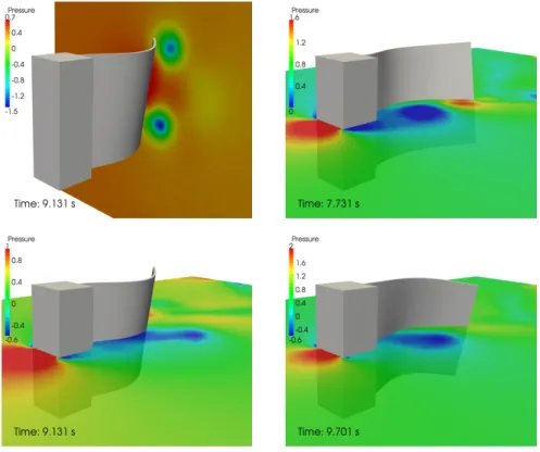
Figure 6: Solution snapshots of flexible plate case. Pressure contours on the planex1 = 4 (top left) andx3= 0 (others), given in Pa.
of the vertical-midpoint at the end of the plate (x1 = 4, x2 = x3 = 0) over the last ten seconds of the simulation, which is 0.734 cm for the coarse mesh and 0.723 cm for the fine mesh; an agreement to within 1.5%. The average frequencies over this same range are 0.970 Hz for the coarse mesh and 0.932 Hz for the fine mesh, a difference of 3.9%. A high degree of mesh independence of the steady-state solution has thus been reached.
It is interesting to compare these results with the equivalent two-dimensional case [22, 55]. In that case, two different regimes of limit-cycle oscillation were observed, the first with an amplitude of approximately 2.0 cm and a frequency of approximately 0.8 Hz, and the second with an amplitude of 0.8 cm and frequency of 2.9 Hz, approximately. These correspond to the first and second mode of vibration of the flexible tail, and depend on initial conditions applied to the flexible tail. In the 3D case analysed here, vibration is in the first mode and the amplitude is almost half of the equivalent 2D case. This is attributable to the fact that pressure can equalise from one side of the plate to the other via flow across its lateral edges. The resulting circulation in the x2–x3 plane is clearly visible in the first panel of Fig. 6. The frequency, on the other hand, is of comparable magnitude, with the discrepancy attributable to the nonlinear
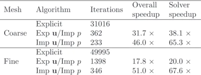
Table 1: Speedup in computation time for a representative timestep of the block-plate problem with two different mesh densities. Number of iterations to convergence are also shown. Overall speedup includes time taken on mesh movement and preprocessing, in contrast to solver speedup.
Mesh Algorithm Iterations Overall Solver speedup speedup Coarse
Explicit 31016
Expu/Impp 362 31.7× 38.1× Impu/Impp 233 46.0× 65.3× Fine
Explicit 49995
Expu/Impp 1398 17.8× 20.0× Impu/Impp 346 51.0× 67.6×
dependence of frequency on amplitude. In the 3D simulation in [68], on the other hand, the plate begins oscillating in its second mode, with a frequency close to 4 Hz and an amplitude of approximately 0.5 cm – also similar to the equivalent 2D results. The fact that we observe a different mode of vibration to that in [68] may be due to initial conditions. In that paper, the plate is kept rigid for the first two seconds of analysis while the flow velocity is ramped up.
This may prevent the plate from receiving the perturbation necessary to excite first-mode vibrations. Also, the form of ramping is different in [68] to that used here. Both results are of much larger amplitude than those reported in [29].
In the second analysis, with the more flexible plate, an inflow velocity of 51.3 cm s−1 was used. A smaller time-step size of ∆t = 0.002 s was selected to account for the faster, second-mode oscillations present in this case. Time- histories of corner displacements are shown in the right-hand panels of Fig. 5, and Fig. 6 shows snapshots of the response with pressure contour colouring. As seen, the higher-frequency second-mode of vibration is excited, with additionally a much larger component of the anti-symmetric twisting mode present. The vortices that drive the oscillations are visible in the right-hand panes of Fig.
6, while in the top-left pane, counter-rotating vortices coming off the corners are visible in the vertical plane. The coarse and fine mesh solutions again show good qualitative agreement once oscillations have grown to limit-cycle state. To quantify this we measure the RMS amplitude of the vertical-midpoint oscillation for 6< t <10 s, obtaining a value of 0.579 cm for the coarse mesh and 0.586 cm for the fine mesh, which constitutes agreement to within 1.2%. For the coarse mesh, the average frequency over this range is 4.95 Hz while for the fine mesh it is 4.90 Hz, a difference of 1.0%.
6.1.1. LU-SGS/GMRES performance speedup
In this section, we analyse the performance improvement effected by the advanced solver algorithms applied to the pressure and momentum equations.
Quoted values are the improvement in overall performance of the FSI solver,
Linear speedup Speedup per iteration Number of iterations
(a)
Number of processors (fluid domain)
Speed-up
200
150
100
50
0 70 60 50 40 30 20 10 0 80 70 60 50 40 30 20 10
0 Linear speedup
Speedup per iteration Number of iterations
(b)
Number of processors (fluid domain)
Numberofiterations
300 250 200 150 100 50 0
140 120 100 80 60 40 20 0 140 120 100 80 60 40 20 0
Figure 7: Parallelisation speed-up for the block-tail problem. (a) Coarse mesh (490 000 cells) and (b) fine mesh (1.6M cells). The right axis depicts the number of fluid iterations required per time-step.
even though the advanced solver is only applied to the fluid subdomain. The number of parallel subdomains used was 23 and 7 for the coarse fluid and solid meshes respectively, increased to 42 and 22 in the case of the fine mesh.
For the purpose of solver speed-up assessment, we have first initialised the block with flexible plate problem by running it for one second in order to reach a representative time-step, and then compared the time taken to reduce the residual at the subsequent time-step by five orders of magnitude. Two ad- vanced solver variants were investigated. Firstly, preconditioned GMRES was applied to the pressure equation with Jacobi iterations used to converge the momentum equations (denoted ‘Exp u/Imp p’ in Table 1). Six Krylov-space vectors were used with three GMRES iterations for each iteration in pseudo- time. The CFL number used was 0.8 for the momentum equations and 1×10⁵ for the pressure equation. Secondly, we considered the momentum equations implicitly by setting β = 1 in Eq. (22) and adding one LU-SGS iteration for each pseudo-timestep (‘Imp u/Imp p’). This allowed the CFL number to be increased to 1.4 for the momentum equations. Both of these algorithms are compared to standard Jacobi used for both pressure and momentum equations (‘Explicit’), where the CFL number was set to 0.8.
The achieved speed-ups are listed in Table 1. Overall solver speed-ups for the full implicit method were around 65 times. It is interesting to note that the speedup effected by the implicit treatment of the pressure in isolation is less for the fine mesh than for the coarse mesh, whereas with implicit velocity relaxation the speedup is very similar in the two cases. This is most likely due to the restriction in timestep size caused by the viscous terms, which is a quadratic function of mesh spacing. Thus, although the pressure equation is treated implicitly, for the finer mesh the viscous timestep restriction begins to become the bottleneck unless the viscous terms are treated implicitly as well.
Figure 8: Meshes used for pipe problem.
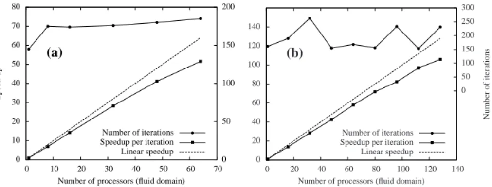
6.1.2. Parallel efficiency
The strong-scaling performance of the entire coupled solver was evaluated by assessing the time taken to complete the first two time-steps of the block with flexible plate problem. The results of the study are depicted in Fig. 7, where the number of iterations achieved per second has been normalised to the value for a single processor. Note that, as a consequence of the preconditioning being done block-for-block on each parallel subdomain, the number of iterations taken to converge the time-step is not constant, and is also plotted in Fig. 7. As seen, this does not show a clear deteriorating trend as one may expect. Also plotted is the speed-up per iteration. After the initial scaling from one to eight cores which is somewhat below linear due to shared-memory bandwidth saturation, the scaling with distributed memory is linear until communication begins to dominate over computation.
6.2. Pressure-pulse in flexible tube
The second test-case comprises a flexible tube 5 cm in length with inner diameter of 1 cm and wall thickness of 0.1 cm. This problem is associated with arterial flow and has been considered by many researchers [27, 70, 71, 72]. It constitutes a worthy test for an incompressible FSI solver as tube flexibility is paramount to the solution. However, a mesh independent solution has never been provided for comparison purposes. Here we aim to establish one, as the problem constitutes a simple and relatively inexpensive test for FSI codes. The walls have densityρs = 1.2 g cm−3 and elastic modulusE = 3×10⁶ g cm−1 s−2. A Poisson’s ratio ofν = 0.3 is used. To model a prototypical liquid, the fluid inside has density 1 g cm−3and a viscosityµ= 3×10⁻²g cm−1s−1. The tube wall is clamped at both ends, with a pressure boundary condition imposed on the fluid at either side. On the left side the pressure is set to 1.3332×10⁴Pa
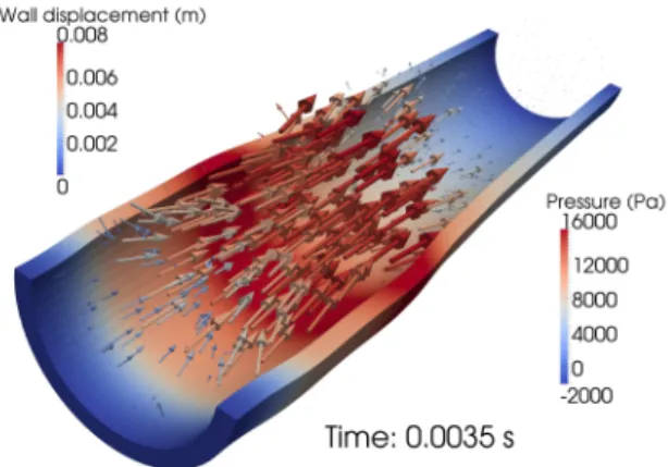
Figure 9: Solution snapshot att= 0.0035 s. Solid deflection is exaggerated by a factor of 10. Velocity vectors are scaled according to velocity magnitude and coloured according to pressure.
fort <0.003 s and zero thereafter, while on the right it is set to zero throughout the analysis. The result is that a pressure wave travels down the tube.
The three computational meshes used are depicted in Fig. 8 and denoted Coarse, Intermediate and Fine. In each case to obtain a finer mesh, the spacing was reduced by a factor of 1.5 in each direction, resulting in a roughly 3.4 times increase in the number of cells. The number of fluid cells is, respectively, 91 000, 301 000 and 1 million for the three meshes, with the solid domain containing 38 000, 130 000 and 454 000 cells respectively. A time-step size of 1×10⁻⁴was used as in [27]. For this problem, the calculation of the redistribution of nodes for mesh movement has to be modified, withD1 andD2 in Eq. (15) taking on the meaning of shortest distance to the solid boundary and shortest distance to the centreline,x=y= 0, respectively.
Figure 9 shows a snapshot of the solution, with wall displacement exagger- ated by a factor of 10 for clarity. Figure 10 depicts the radial components of displacement and velocity of the pipe wall at a point on the inner wall halfway along the pipe. It is evident that the fine mesh result is close to converged, with the maximum change in velocity between the coarse and intermediate meshes of 8.2% in peak velocity reducing to 3.4% between the intermediate and fine meshes. The coarse mesh analysis completed in 125 minutes using four Intel Core 2 2.66 GHz computational cores, while the finest mesh took 938 minutes using 31 AMD Opteron 800 MHz cores.
7. Conclusion
A fast parallel strongly-coupled partitioned FSI scheme was developed us- ing a 3D edge-based finite volume methodology. Laminar incompressible flows interacting with structures undergoing large non-linear displacements were con- sidered. The incompressible fluid divergence constraint was dealt with using
Fine Medium Coarse
Time (s)
Displacement(m)
0.01 0.008 0.006 0.004 0.002 0 0.01 0.008 0.006 0.004 0.002 0 -0.002 -0.004
Fine Medium Coarse
Time (s) Velocity(ms−1)
0.01 0.008 0.006 0.004 0.002 0
6 4 2 0 -2 -4 -6 -8
Figure 10: Radial component of dispacement (left) and velocity (right) of the inner tube wall at half the length of the pipe. Solutions are shown for the three mesh densities given in the text.
a new artificial-compressibility algorithm stabilised with Consistent Numerical Fluxes. The fluid solver was accelerated via the implicit treatment of pressures in the continuity equation and implicit treatment of viscous terms in the mo- mentum equations. These were respectively solved via two matrix-free methods viz. LU-SGS preconditioned GMRES and LU-SGS. The solver was parallelised using METIS and MPI for distributed memory architectures. Two strongly- coupled test problems were considered, and solver performance assessed via mesh indepedance studies. A high degree of mesh indepedance was demon- strated throughout. Advanced solver computational performance demonstrated truly fast and efficient parallel solution. Overall speed-ups achieved were circa 50 while ensuring linear distributed parallel-scaling for up to 128 CPUs for the problems considered.
Acknowledgements
The authors wish to thank the Centre for High Performance Computing (CHPC) for access to computing hardware. This work was funded by the Coun- cil for Scientific and Industrial Research (CSIR) on Thematic Type A Grant nr.
TA-2009-013.
References
[1] R. M. Bennet, J. W. Edwards, An overview of recent developments in com- putational aeroelasticity, in: Proceedings of the 29th AIAA fluid dynamics conference, Albuquerque, NM, 1998.
[2] C. Farhat, K. G. van der Zee, P. Geuzaine, Provably second-order time- accurate loosely-coupled solution algorithms for transient nonlinear com- putational aeroelasticity, Computer Methods in Applied Mechanics and Engineering 195 (2006) 1973–2001.
![Figure 4: Meshes used for block with flexible plate. Coarse mesh [(a) and (b)] and fine mesh (c).](https://thumb-ap.123doks.com/thumbv2/pubpdfnet/10463881.0/17.892.201.711.182.643/figure-meshes-used-block-flexible-plate-coarse-mesh.webp)