The effect of the variable chaplygin gas on the CMB.

(1)

The Effect of the Variable Chaplygin Gas on the CMB

Sphesihle Makhathini University of KwaZulu-Natal School of Physics and Chemistry

Supervisor : Dr. Caroline Zunckel

A Thesis submitted in part fulfilment of the degree of MSc in Physics at the

University of KwaZulu-Natal 2013

As the candidate’s supervisor I have approved this dissertation for submission:

Signed : Name: Caroline Zunckel Date 25 April 2013

As the candidate’s supervisor I have approved this dissertation for submission:

(2)

2

Declaration

I, Sphesihle Makhathini, declare that

• The research reported in this dissertation, except where otherwise indicated, is my original research.

• This dissertation has not been submitted for any degree or examination at any other university.

• This dissertation does not contain other persons data, pictures, graphs or other information, unless specifically acknowledged as being sourced from other persons.

• This dissertation does not contain other persons’ writing, unless specifically acknowledged as being sourced from other researchers.

• This dissertation does not contain text, graphics or tables copied and pasted from the Internet, unless specifically acknowledged, and the source being de- tailed in the dissertation and in the References sections.

Signed :

(3)

3

Abstract

In this dissertation, we consider the variable chaplygin gas (VCG) model as derived from the Tachyon gas model and search for a sub-class of models that provide an adequate fit to the cosmic microwave background (CMB) observations. We find that, for an appropriate choice of VCG parameters, up to ∼ 80% of the VCG collapses into a gravitationally bound condensate which behaves as matter; the evolution of the remaining VCG, as governed by its equation of state, brings about accelerated expansion at late times. In light of this high collapsed fraction, we approximate the VCG transfer function with that of cold dark matter. We show that we can sufficiently describe the VCG cosmology from decoupling to today in terms of a model in which the gravitationally bound condensate plays the role of cold dark matter and the remaining VCG takes the place of dark energy in the concordance model. We then compute the CMB temperature anisotropy spectrum for a subset of VCG models and proceed to find a best-fit model to the WMAP-9yr data [46]. Our best-fit model has a χ² per degrees of freedom of 2.03.

Acknowledgements

First and foremost, I would like thank my supervisor Caroline Zunckel for believing in my ability to finish this project. She has taught me how to think like a scientist and how to express my thoughts in a logical way. I am also very grateful to Robert Lindebaum for all the support and guidance with which he provided me.

In addition, I would also like to thank my family for their unfailing support throughout my academic career. Last but not least, I would like to thank the National Institute for Theoretical Physics (Nithep) for funding my postgraduate education thus far.

(4)

Chapter 1 Introduction

With the advances in observational and theoretical cosmology, in recent years, ques- tions about the age, geometry, dynamics, content, and the origin of the structure in the universe can be answered quantitatively with reasonable confidence. We know that the very early universe was in an extremely hot state which expanded rapidly, causing it to cool, and resulting in the present expanding state. Current cosmological observations suggest that we live in an almost spatially flat, expanding universe with about 70% percent of the energy density attributed to a component with negative pressure, dubbed dark energy. The remainder of the energy density is attributed to 25% non-baryonic matter, known as dark matter, and about 5%

baryonic matter.

This cosmological model is known as the ΛCDM model. The ΛCDM model supposes that dark energy is Einstein’s cosmological constant, while dark matter particles are assumed to non-relativistic, cold dark matter (CDM). However, despite the consistency with most observations, the ΛCDM model has encountered some theoretical problems [54]. Furthermore, neither dark matter nor dark energy has been directly detected. This leaves the door open to the possibility that dark matter and dark energy are manifestations of the same cosmic fluid. This scenario, where dark matter and dark energy are manifestations of the same cosmic fluid is calledQuartessence.

In light of the challenges facing ΛCDM it is important to explore such a scenario.

In this dissertation, we investigate the possibility of a quartessence model known as the variable Chaplygin gas (VCG) as a viable alternate cosmology to ΛCDM in light of the current observational data.

In this introduction we first describe the theory that governs the dynamics of the universe. Then we give a description of the current cosmological observations and how these observations have led to the current concordance model. Most of this background material is based on references [1, 2, 3]. Finally we present quartessence as a possible alternative to ΛCDM.

1.1 Describing the Universe

In this section we present a qualitative description of the theoretical framework that describes the dynamics of our universe.

6

(7)

1.1. DESCRIBING THE UNIVERSE 7

1.1.1 Equations of Motion

The universe is believed to be isotropic and homogeneous, the so-called cosmological principle. Isotropy means that the universe looks the same in every direction, which then implies that observations made in one direction are a sufficient test of cosmology. Isotropy is in very good agreement with observations (0.001% accuracy).

Homogeneity means the general picture of the universe as a function of time is independent of the position of the observer. The assertion of the cosmological principle together with General Relativity describes our universe. General Relativity relates the metric, which describes gravitation, to the energy in the universe through the Einstein equations, which determine the dynamics of the universe:

G_µν =R_µν −1

2g_µνR= 8πGT_µν, (1.1)

whereGµν is the Einstein tensor;Rµν is the Ricci tensor, which depends on the metric derivatives; the Ricci scalar R is a contraction of the Ricci tensor, R=g^µνR_µν; Gis Newton’s gravitational constant; andT_µν is the energy-momentum tensor. The metric,gµν, which describes a smooth expanding universe is the Friedman-Lemaitre- Robertson-Walker (FRW) metric

ds² =dt²−a(t)[dr²+S_κ(r)²dΩ²], (1.2) wherea(t) is the scale factor. It is conventional to set its value today to unity and its value at the Big Bang to be zero;dΩ² =dθ²+ sin²(θ)dφ² and

S_κ =







p1

κsin(r√

κ) for κ >0

r κ = 0

p1

κsinh(r√

κ) forκ <0







. (1.3)

Here, κ denotes the curvature of the universe and can be either positive, zero or negative depending on the geometry of the universe. A flat universe is Euclidean and has zero curvature: particles remain parallel as long as they travel freely. In an open universe which has negative curvature, particles which start out parallel gradually diverge as they travel freely. In a closed universe, which has positive curvature;

particles which start out parallel gradually converge as they travel freely.

The left hand side of (1.1) is a function of the metric and the right a function of the energy. Assuming each component in the universe has an energy densityρ_i and pressurep_i, the total energy density and pressure are given by

ρ = X

i

ρ_i (1.4)

p = X

i

pi, (1.5)

respectively. For a perfect isotropic fluid the energy-momentum tensor is given by

T^µ_ν =







−ρ 0 0 0

0 p 0 0

0 0 p 0

0 0 0 p







, (1.6)

(8)

8 CHAPTER 1. INTRODUCTION wherepis the pressure of the fluid with energy density ρ. For a perfect fluid energy conservation requires

T^µν_;µ = 0, (1.7)

which yields as its longitudinal part the continuity equation

∂ρ

∂t + 3a˙

a(ρ+p) = 0. (1.8)

The continuity equation can then be integrated to get the evolution of the energy density for each component as

ρ_i ∝exp

−3 Z a

da⁰

a⁰ [1 +w_i(a⁰)]

(1.9) wherew_i(a) is the equation of state parameter, defined as

wi = pi

ρ_i. (1.10)

Knowing the equation of state parameter for a given component in the universe, the energy density evolution of each component can be obtained using Equation (1.9).

The Einstein equations yields the evolution of ˙a as

− a˙

a 2

+8πG 3 ρ+ κ

a² = 0, (1.11)

and ¨a is given by

¨ a

a +4πG

3 (ρ+ 3p) = 0. (1.12)

Therefore, for a universe containing fluids with known equation of state parameters w_i, the dynamics are described by equations (1.9),(1.11) and (1.12). Equation (1.11) is known as the Friedman equation. To quantify the change in the scale factor and its relation to the energy, it is useful to define the Hubble parameter,

H = 1 a

da dt = a˙

a. (1.13)

Now the Friedman equation can be written using the Hubble parameter as

−H²+8πG 3 ρ+ κ

a² = 0. (1.14)

Another quantity that is frequently used in cosmology is the redshift, which is defined as the ratio of the wavelength when light was observed and light was emitted, i.e,

z+ 1 = λ_observed λ_emitted = 1

a. (1.15)

Redshift is often used as a time and distance parameter in cosmology. The redshift of the light emitted by source at time t_i, z_i =a(t) ¹, gives the size of the universe at the timet_i.

(9)

1.2. EVIDENCE FOR THE BIG BANG MODEL 9

1.2 Evidence for the Big Bang Model

In this section we describe the current cosmological observations. In this description we highlight the role each these observations play in validating the Big Bang Model. We then proceed to study how these observations have led to the current concordance model universe.

1.2.1 The Hubble Expansion

One giant leap in understanding the dynamics of the universe was Edwin Hubble’s discovery that the universe is expanding. Using the 100-inch Hooker telescope at Mount Wilkinson Observatory Hubble measured distances to galaxies by isolating individual Cepheids in those galaxies. Cepheids are stars which pulsate. The period of their pulsation is related to their intrinsic brightness. Cepheids with same period have the same intrinsic luminosity. Distances to these objects can be inferred by finding the correlation between their true and observed brightness. Hubble combined his measurements with Veto Slipher’s redshift measurements for the galaxies, which may be determined by measuring the shifts of spectral lines in spectra from galaxies. He found that galaxy redshifts were proportional to galaxy distances, and concluded that these galaxies were receding from us with a velocity proportional to their distance from us. According to the cosmological principle we hold no special place in the universe, therefore it must be that galaxies recede from each other with a velocity v, proportional to the distance, r, between them. This relation is known as the Hubble law:

v =H0r. (1.16)

The constantH₀ is referred to as the Hubble constant and is a measure of the rate of the recession. Present measures of the Hubble rate are parametrised by h, defined via,

H₀ = 100hkm s ¹ Mpc ¹. (1.17)

The Hubble law remains one of most compelling pieces of evidence that the universe is expanding, which is consistent with the Big Bang model. Therefore accurate measurement of the expansion rate is paramount. The standard candles that are used today are Type Ia supernovae (SN1a), being much brighter than Cepheids they can extend the Hubble diagram 1.1a to very large redshifts 1.1b, and measure the expansion rate to a very high accuracy. very

(10)

10 CHAPTER 1. INTRODUCTION

(a) The original Hubble diagram, showing the velocities of galaxies vs distance, taken from [4]. The solid line is the line of best-fit for data points (filled) corrected for the motion of the sun, while the dashed line is the best-fit for the uncorrected data points (unfilled).

(b) Hubble Diagram from the Hubble Space Telescope Key Project [5], constructed from five different distance measures. The horizon lines give the best-fit value ofH₀= 72±8km s ¹Mpc ¹.

Figure 1.1

(11)

1.2. EVIDENCE FOR THE BIG BANG MODEL 11

1.2.2 Light Element Abundance

The abundance of elements in the universe provides one of the most compelling pieces of evidence in support of the Big Bang model. Historically it was assumed that all stars began their life comprised entirely of hydrogen, with heavier elements being generated via nuclear fusion reactions at their cores. While this is the process giving rise to heavy elements, it is now established that not all the light elements–

deuterium, helium-3, lithium, and especially helium-4, could have been created in this manner. In fact the spectra of very young stars indicates these approach non-zero abundances. In particular, the measurement of primordial deuterium pins down the baryon density extremely accurately to only a few percent of the critical density.

Figure 1.2: Constraints on the baryon density as predicted by BBN taken from [6].

The curves show the primordial abundances of deuterium, helium-3, lithium and helium-4 as predicted by the standard model of the BBN, as function of baryon density-photon ratio. The boxes show the observed abundances.

(12)

12 CHAPTER 1. INTRODUCTION When the universe was much hotter and denser, when the temperature was of order ∼ 10 MeV, there were no neutral atoms or even bound nuclei. The vast amounts of radiation in such a hot environment ensured that any atom or nucleus produced would be immediately destroyed by a high energy photon. However, according to the Big Bang model, as the universe cooled well below binding energies of typical nuclei (∼1MeV), the production of light elements could take place. This period when neutral nuclei began to form is referred to as therecombination epoch.

Knowing the conditions of the early universe and the relevant nuclear cross-sections (standard model of particle physics), one can predict the expected primordial abundances of Li, He and D in this model. This synthesis of light elements is known as Big Bang Nucleosythesis (BBN). The predictions of BBN are in very good agreement with the current estimates of light element predictions, and this consistency sets the Big Bang model on an even firmer footing. The combined proton-neutron density is called the baryon density since both protons and neutrons have baryon number one and these are the only baryons around at these early times. Thus BBN may be used to measure the baryon density in the universe (see section 1.3).

1.2.3 Cosmic Microwave Background

During the epoch of recombination, photons are coupled to baryons. Cosmic expansion causes the baryon density to decrease causing a decrease in photon-baryon interaction. When the photon-baryon interaction rate decreases below the cosmic expansion rate, the photons are decoupled from the baryons and begin to free- stream. George Gamow in 1948 predicted that this primordial radiation should be present today with an almost perfect uniformity everywhere in the universe. In the early 1960s this primordial radiation was recognised by Robert Dicke and Yakov Zeldovich as a detectable phenomenon.

In 1965, Arno Penzias and Robert Wilson at the Bell Telephone Laboratories in New Jersey were measuring sky brightness at radio wavelengths. Their measurements had an excess of 3.5 K which they could not account for. When Penzias and Wilson heard of Dicke’s work they realised they had detected the CMB. In 1990 satellite measurements confirmed the CMB has a blackbody spectral distribution with an apparent temperature of 2.7 K. As a result of the continual expansion of the universe, this radiation has been stretched out to longer wavelengths which today exist in the microwave region of the electromagnetic spectrum. Due to its near perfect uniformity, we conclude that this radiation originated in a time when the universe was much smaller, hotter, and denser.

1.3 Cosmic Budget

One major goal in observational cosmology is to know the precisely the fraction contribution of each component of the universe. Observations and theory point to a universe made up of radiation,ρ_γ, baryonic matter (electrons, neutrons, protons), ρ_b, dark matter,ρ_dm, dark energy,ρ_de and neutrinosρ_nu. In this section we calculate the contribution of each of the above mentioned species to the energy density of the universe. Before we proceed we need to define the critical density. Note that in a

(13)

1.3. COSMIC BUDGET 13 flat universe (κ= 0) the Friedman equation (1.14) becomes

−H²+8πG

3 ρ= 0 (1.18)

which leads to the definition of the critical density ρ_cr = 3H²

8πG. (1.19)

Equation (1.19) says that, in a flat universe, the total energy density isρ_cr, i.e, in a universe with M components the total energy is

ρ_cr =

M

X

i

ρ_i. (1.20)

To facilitate comparison between the difference in contributions made by each component to the total energy density, it is useful to define the density parameter, which is a dimensionless quantity

Ω_i = ρ_i

ρ_cr, (1.21)

and is the fractional contribution of the different components to the energy density of the universe (With the total energy density comprising the sum of all con- stituents). For a flat universe, Ω = 1. In this dissertation, we denote values of cosmological parameters today with a “0” subscript.

Matter

Matter effectively has zero pressure, and therefore its equation of state parameter wm, vanishes, so that the matter energy density scales as

ρ_m(a)∝exp

−3

Z a da⁰ a⁰

=a ³. (1.22)

Observations point to the existence of non-baryonic matter, also referred to non- luminous matter since it does not interact in any significant way with radiation.

The matter contribution is therefore, Ω_m = Ω_b + Ω_dm. Baryons

Current estimates of the baryon density constrain the baryon density to ∼2−5%

of the critical density. BBN, which has already been discussed in section 1.2.2, constrains the baryon density to Ω_b,0h² = 0.020±0.002 [51]. Another approach is to look at spectra of distant galaxies, and measuring the amount of light absorption.

The amount of light absorbed quantifies the amount of hydrogen the light encounters along the way, the baryon density is then inferred from the estimate of the amount of hydrogen. This approach roughly estimates Ω_b,0h² ' 0.020 [29]. One can also compute the baryon content of the Universe from the anisotropies of the CMB radiation. This approach puts fairly stringent limits on the baryon content to about Ω_b,0h² = 0.024^+0.004_0.003 [45].

(14)

14 CHAPTER 1. INTRODUCTION Dark Matter

The matter density of a system may also be measured by studying the gravitational field produced by the matter in that system. In the case of spiral galaxies, one can measure the rotation of a galaxy at different distances from its centre and plot the rotational velocity against the distance, the so-called rotational curve. The gravitational field due to spiral galaxies can then be determined by studying their rotational curves. However, this technique estimates about 80% more matter than that inferred from the spectra of these galaxies, pointing to the existence of non- luminous matter. Furthermore, non-luminous estimates of the luminous/baryonic matter predict the matter density to be 20−30%. One of these techniques uses a phenomena predicted by general relativity– the trajectory of a photon is affected by the curvature of space-time induced by the presence of a massive object (the “lens”)–

known as gravitational lensing. Current gravitational lensing measurements of the matter density constrain it to Ω_m,0 = 0.248±0.019 [51]. Clusters of galaxies, which are the largest known objects, are likely to be representative of the matter in the universe. Therefore, measurements of the baryon to matter ratio in these objects combined with good estimates of the baryonic matter density will give estimates of the dark matter density. The baryon to matter ratio in these objects is roughly 20%. One could also infer the matter density by looking at CMB anisotropies, which constraints the matter density to Ω_m,0h² = 0.1326 ±0.00063 [45]. These independent methods provide compelling evidence that the baryon density is of order of 5% of the critical density, while the total matter density is about five times larger, providing clear evidence for non-baryonic matter. However, dark matter has not been detected directly and all the current evidence is based on its gravitational effects. Currently the most viable candidate for dark matter is known ascold dark matter (CDM), which is mostly composed of non-relativistic particles, although, theory also allows for dark matter composed of relativistic particles; hot dark matter (HDM). However, relativistic particles cannot clump together easily, and therefore could not have stimulated the formation of small (on cosmological scales) structures like galaxies and clusters of galaxies. Therefore, dark matter particles are predicted to move slowly to allow them to clump to form the dark matter halos that give the structure of the universe. As a candidate for the CDM particle, the particle physics inspired weakly interacting particle (WIMP) was proposed. WIMPs are postulated to interact mainly through the weak force and gravity, but not through the electromagnetic force, making them the prime candidates for DM particles.

Dark Energy

With matter (baryonic and non-baryonic) making up∼27% of the critical density and indications of spatial flatness, there is clearly a shortfall in the energy density budget. This points to another component in the universe that makes up about two- thirds of the critical density. Furthermore, in 1998, two independent groups (Riess et al. 1998 [30], Perlmutter et al. 1999 [31]) observed a group of SNIa standard candles to be fainter than expected in a matter dominated universe. The manner in which the brightness of standard candles evolves with redshift provides information about the evolution of the universe at late times. Their results are indicative of an

(15)

1.4. QUARTESSENCE AN ALTERNATIVE TOΛCDM 15 accelerated expansion rate. Since all known matter is attractive, a component with a negative pressure is therefore believed to be driving the accelerated expansion rate. This component is believed to be the cosmological constant which was first introduced by Einstein in order avoid the non-static universe predicted by his theory of General Relativity. The pressure of this component is given by

pΛ=−ρΛ. (1.23)

Λ has been interpreted as vacuum energy; in quantum physics one possible origin is a type of ‘zero-point energy’, which remains even in the absence of matter. The density of the cosmological constant, ρΛ, is constant throughout the evolution of the universe, i.e., Λ(t) = constant. This component has been shown to give rise to the accelerated expansion phase detected by SNIa observations.

Currently the best estimates for the cosmic budget are the WMAP [45] values:

Ω_de,0 = 0.734±0.029, Ω_dm,0 = 0.222±0.026, Ω_b,0 = 0.0449±0.0028.

1.4 Quartessence an Alternative to ΛCDM

The ΛCDM model accounts for a wide range of observations, but encounters two theoretical issues. Firstly, according to the standard model of particle physics, Λ must have tiny energy density (∼ 10 ⁴⁷ GeV ⁴ ). This requirement for a fine- tuned value of Λ, is called the fine-tuning problem. The second problems arises when the ΛCDM model is extrapolated back in time to the very early Universe.

The dark energy density decreases at a different rate from the matter density, and their ratio shrinks by many orders of magnitude as we extrapolate back in time.

Now, the ΛCDM model predicts the ratio was set initially just right so that today, some fourteen billion years later, the ratio is of order unity. It is a remarkable coincidence that somehow we exist in this small (on cosmological scales) epoch when Ω_Λ/Ω_m ∼1. This is known as the coincidence problem. To address the fine tuning and coincidence problems many other models have been proposed, most of which propose a dynamic dark energy. Dynamical dark energy models have a time varying dark energy component, Λ(t). Among these, quintessence [7, 8], holographic dark energy [10], quintom [9] and phantom [11] are the most famous. These models attempt to address the fine-tuning problem that arises from the ΛCDM model, and provide a satisfactory fit to observations. However like the ΛCDM model, these models treat dark matter and dark energy as separate entities. However, since there has been no direct detection of either dark matter or dark energy, a scenario where dark dark matter and dark energy are manifestations of the same cosmic fluid has been sought. Such a scenario is called Quartessence or unified dark mater, dark energy (UDME). The Chaplygin gas [19, 39], which is a fluid with an exotic equation of state, provides an interesting quartessence scenario. The redshift dependence of this gas is such that at high redshifts (early times), it behaves like matter and low redshift (late times) it behaves like dark energy. However, to successfully model the universe, a sufficient fraction of this fluid has to condense into a gravitationally bound condensate in order to account for structure in the universe. In this dissertation we will study a version of the Chaplygin gas, known

(16)

16 CHAPTER 1. INTRODUCTION as the variable Chaplygin gas, in light of the CMB observations. Other variations of the Chaplygin gas exist, namely, the Generalised Chaplygin gas [39] and the Modified Chaplygin gas [14]. However, unlike the standard Chaplygin gas, these variations do not have an equivalent brane interpretation [12].

1.5 About This Thesis

In Chapter 2, we describe the growth of the primordial density perturbations. We start with a Newtonian formalism for the growth of a spherically symmetric overdensity and then move on to formulate a fully General Relativistic model for a spherically symmetric space-time. We then apply this model to a single fluid model.

In Chapter 3, we study how the observed CMB and matter power spectra can be used to test the validity of cosmological models. In Chapter 4, we introduce the idea of quartessence, in particular the Chaplygin gas. We also describe the evolution of the inhomogeneous variable Chaplygin gas. In chapter 5, we first calculate the fraction of VCG that collapses into a gravitationally bound condensate. We then move on to formulate our VCG cosmology. We also describe the FORTRAN 90 code used to do the calculations. In Chapter 6 we discuss the the effects of the VCG on the CMB spectrum and finally in chapter 7 we make our concluding remarks.

(17)

Chapter 2

Cosmological Perturbations

The cosmological principle holds on cosmological scales. On smaller scales however, the universe contains density fluctuations ranging from planets to large super clusters and voids. On smaller scales homogeneity and isotropy are clearly violated.

This violation of the cosmological principle may be explained by supposing that, in its infancy, the primordial density fluctuations were very close to smooth, with tiny density fluctuations. These tiny density fluctuations have grown by gravitational instability to bring about the complex structure we observe today. As for the origin of the tiny density fluctuations, the widely accepted hypothesis assumes they are quantum fluctuations amplified by a brief period of exponential expansion, known as inflation. In this section we study the evolution of the primordial density field.

The material in this chapter is based on references [1, 2].

2.1 Formation of Structure

In this section we describe growth of structure. We first describe a linear approach using Newtonian theory, and then we describe a General Relativistic approach to gravitational collapse.

2.1.1 Gravitational Instability

Consider some component of the universe with energy densityρ(r, t), which depends on position and time. The spatially averaged energy density, at a given time, averaged over some volume V; which is much larger than the largest structure in the universe, is

ρ= 1 V

Z

V

ρ(r, t)d³r. (2.1)

The density contrast is defined as

δ(r, t) = ρ(r, t)−ρ(r, t)

ρ(r, t) . (2.2)

In overdense regions,δ >0, andδ <0 in underdense regions. The density contrast is a minimum, δ=−1, when ρ= 0, and there is no definite upper limit on δ. The

17

(18)

18 CHAPTER 2. COSMOLOGICAL PERTURBATIONS study of the growth of structure requires knowing how small density perturbations δ 1, grow in amplitude under the influence of gravity. Before we continue it is useful to define the Jeans Length in a context of a expanding universe. Consider a spherical overdensity with radiusR. In the absence of pressure, the time scale for collapse is

t_dyn ∼(Gρ) ^1/2. (2.3)

In the presence of pressure, collapse will be countered by steepening of the pressure gradient within the perturbation. The steepening, however, is not instantaneous, since any changes in pressure travel at the local (of the perturbation) sound speed, c_s. Thus the time it takes for the pressure to build up is

tpre ∼ R

c_s . (2.4)

Hydrostatic equilibrium requires the pressure gradient to build up before the overdense region collapses, i.e., the time it takes for the pressure to build up must be less than the collapse time scale. Considering equations (2.3) and (2.4), one can conclude that for a density perturbation to be stabilised by pressure against collapse, it must be smaller by some characteristic sizeλ_J, the so-called Jeans Length λ_J ∼c_st_dyn ∼(Gρ) ^1/2, (2.5) including all the factors ofπ, the Jeans Length is

λ_J = 2πc_st_dyn. (2.6)

Overdense regions of scales larger than the Jeans length will collapse under their own gravity, while regions smaller than the Jeans length oscillate in density. Now consider a flat expanding universe with average density ρ, and with fluctuations of amplitude |δ| 1. The characteristic time for expansion in such a universe is the Hubble time,

H ¹ =

3c² 8πGρ

1/2

, (2.7)

which, together with equation (2.3), leads to H ¹ =

3 2

1/2

tdyn. (2.8)

The Jeans length in an expanding universe therefore becomes λ_J = 2πc_st_dyn = 2π

3 2

1/2

c_s

H . (2.9)

2.1.2 A Newtonian Approach

A Newtonian approach is sufficient to study the growth of small perturbations in a flat expanding universe. Consider a matter filled universe, with density ρ(r, t).

(19)

2.1. FORMATION OF STRUCTURE 19 Within a spherical slightly (δ1) overdense region of radiusR, the density within the sphere is

ρ(t) = ρ(t)[1 +δ(t)]. (2.10) The total gravitational acceleration at the surface of the sphere is

R¨ =−GM

R² =−G R

4π

3 ρR³ =−4π

3 GR(ρ+δρ) . (2.11) The equation of motion for a point at surface of the sphere is

R¨

R =−4π

3 G(ρ+δρ). (2.12)

Mass conservation requires the mass inside the sphere M = 4π

3 ρ(t)[1 +δ(t)]R³(t), (2.13) to remain constant as the universe expands, leading to

R(t)∝ρ(t) ^1/3[1 +δ(t)] ^1/3. (2.14) Since this universe is matter-dominated,ρ∝a ³, we also have

R(t)∝a(t)[1 +δ(t)] ^1/3. (2.15) Equation (2.15) implies that if the sphere is slightly overdense, its radius will grow slightly less rapidly than the scale factor. If the sphere is slightly is slightly underdense it will grow slightly more rapidly than the scale factor. The time derivative of (2.15) is

R˙ ∝a[1 +˙ δ] ^1/3− 1

3a[1 +δ] ^4/3δ ,˙ (2.16) and the second time derivative is

R¨ ∝¨a[1 +δ] ^1/3− 2

3a[1 +˙ δ] ^4/3δ

1− 2

3[1 +δ] ¹δ

− 1

3[1 +δ] ^4/3δ .¨ (2.17) Considering thatδ 1, then dividing by equation (2.15) yields

R¨ R ' ¨a

a − 1 3

δ¨−2 3

˙ a a

δ ,˙ (2.18)

then (2.12) and (2.18) lead to the acceleration equation for a such a slightly per- turbed matter-dominated homogeneous, isotropic universe,

¨ a a − 1

3 δ¨− 2

3

˙ a a

δ˙=−4π

3 G(ρ+δρ), (2.19)

which, whenδ = 0, reduces to the acceleration for a homogeneous, isotropic matter- dominated universe

¨ a

a =−4π

3 Gρ . (2.20)

(20)

20 CHAPTER 2. COSMOLOGICAL PERTURBATIONS To find an expression that describes how small perturbations grow, equation (2.20) may be subtracted from equation (2.19) leaving only terms linear in δ:

1 3

δ¨+ 2 3

˙ a a

δ˙= 4π

3 Gδρ (2.21)

or, using equation (1.13)

δ¨+ 2Hδ˙= 4πGδρ. (2.22)

This form of the equation can be applied to a universe with non-negligible pressure, such as the cosmological constant. However in a multi-component universe, δ rep- resents the fluctuations only in the matter density. Equation (2.22) may be written in terms of the matter density parameter,

δ¨+ 2Hδ˙− 3

2Ω_mH²δ = 0. (2.23)

During epochs when matter does not dominate the universe,δdoes not grow rapidly in amplitude. For instance, during the radiation domination era(H = 1/2t, Ω 1), equation (2.23) becomes

δ¨+1 t

δ˙ ≈0, (2.24)

which has solution

δ(t)≈B₁+B₂ln(t). (2.25)

During radiation dominance, the matter perturbations grow at a logarithmic rate.

And more recently, during the dark energy (cosmological constant) domination era, equation (2.23) becomes

δ¨+ 2H_Λδ˙≈0, (2.26)

with solution

δ(t)≈C₁+C₂e ^2H^Λ^t. (2.27) In a Λ-dominated universe, the matter fluctuations asymptotically approach a constant fractional amplitude. When matter-dominates the energy density of the universe, there is a significant growth in the amplitude of the density fluctuations. In this case, H = 2/3t, Ω_m = 1:

δ¨+ 4 3t

δ˙− 2

3t²δ = 0, (2.28)

One may try a power-law solution of the formδ(t) =Dtⁿ, n(n−1)Dtⁿ ²+ 4

3tnDtⁿ ¹− 2

3t²Dtⁿ = 0, (2.29) or

n(n−1) + 4 3n−2

3 = 0. (2.30)

This quadratic equation has solution, n=−1,2/3, giving general solution

δ(t) = D₁t^2/3+D₂t ¹. (2.31)

(21)

2.1. FORMATION OF STRUCTURE 21 The initial conditions for δ(t) can be used to determine, D₁, D₂. The decaying mode D₂t ¹ eventually becomes insignificant compared to the growing mode d₁t^2/3 as t grows. It is worth remembering that this evolution of the density fluctuations holds as long δ 1. When δ ∼ 1, the above approach becomes unreliable to study the evolution of density fluctuations. To study the evolution of δ ∼ 1 and δ > 1 computer simulations can be used. In these simulations, when a region reaches an overdensity δ ∼ 1, it breaks away from the Hubble flow and collapses.

The overdense region oscillates a few times then and attains viral equilibrium as gravitationally bound structure. Baryonic matter evolves to form the stellar part of galaxies, while the dark-matter forms the dark halos within which the stellar components of galaxies are embedded [1].

2.1.3 A Full GR Approach

In this section we describe a spherically symmetric inhomogeneity. We mainly follow the full General Relativistic formalism presented in [12]. The space-time of a spherically symmetric inhomogeneity is described by the metric [12]

ds² =N(t, r)²dt²−b(t, r)²(dr²+r²S_κ(t, r)dΩ²), (2.32) where N is the local lapse function, b is the local expansion factor and S_κ(t, r) describes spatial curvature. In the limit r → ∞, the above metric approaches the FRW metric, i.e., N(r, t) →1, S_κ → 1 and b(r, t) → a(t). The Hubble parameter in a space-time described by the metric (2.32) is given by [12]

H = 1 N

b_,0 b + 1

3 S_κ_,0

S_κ

(2.33) and the shear is given by

σ² = 2 3

1 2N

S_κ_,0 S_κ

2

. (2.34)

Assuming the density contrast to be of fixed Gaussian shape with comoving sizeR, the energy density evolves as

ρ(t, r) = ¯ρ(t)[1 +δ(t, R)e ^r²^/(2R²⁾]. (2.35) The density contrast is given by

δ(a) = ρ(a)−ρ(a)¯

ρ(a)¯ , (2.36)

where background quantities are bared. Since every region is treated as being independent in spherical models, the spatial derivatives of N, ρ, b vanish at the origin. Hence we may expandb and N about the origin as follows

N(r, t) = N(t,0)

1 +O(r²))

(2.37) b(r, t) = b(t,0)

1 +O(r²))

. (2.38)

(22)

22 CHAPTER 2. COSMOLOGICAL PERTURBATIONS Now, evaluating Einstein’s equationG⁰₁ = 0 leads to [12]

2b_,1 b + b_,1

b

S_κ_,0

S_κ −2b_,0 b

− N_,1 N

2b_,0

b + S_κ_,0 S_κ

+ S_κ_,0

S_κ 1

r − 1 2

S_κ_,1 S_κ

= 0. (2.39)

Recalling that the first three terms vanish at origin, the above equality holds only if ^S_S^κ,0

κ = 0 at the origin. Looking at Equation (2.34) we see that the shear vanishes at the origin.

For a one-component model, the Raychaudhury equation

3 ˙H+ 3H²+σ_µνσ^µν+u^µu^ν R_µν = ˙u^µ_;µ. (2.40) combines with Einsteins equations (1.1) to give [12]

3 ˙H+ 3H²+σ²+ 4πG(ρ+ 3p) =

c²_sh^µνρ_,ν p+ρ

;µ

. (2.41)

Evaluating this equation at the origin we get 1

N(t,0)

dH(t,0)

dt +H(t,0)²+ 4πG

3 (ρ(t) + 3p(t)) = c²_s(ρ(t)−ρ(t))¯

b(t,0)²R²(p(t) +ρ(t)). (2.42) From now on we denote the inhomogeneity quantities evaluated at the origin as, H(t,0) =H, b(t,0) = 0, N(t,0) =N. Therefore we rewrite Equation (2.42) as

1 N

dH

dt +H²+4πG

3 (ρ+ 3p) = c²_s δρ¯

b²R²(p+ρ). (2.43) The evolution of ρ(t) may described the continuity equation

dρ

dt + 3H(ρ+p) = 0. (2.44)

Then with an equation of state p = p(ρ), the growth of a spherically symmetric inhomogeneity of a one-component fluid is described by Equations (2.43) and (2.44).

Looking at Equation (2.33), the Hubble parameter evaluated at the origin is H = 1

b db

dt . (2.45)

(23)

2.1. FORMATION OF STRUCTURE 23

2.1.4 Statistics of Collapsed Objects: The Press-Schechter Theory

Up to this point, we have discussed a theory that describes the evolution of the density fluctuations set up during inflation. However, thus far, the theory cannot predict the fraction of matter that has collapsed into non-linear structure. For instance, one may predict the matter distribution in the universe but cannot predict the number density of galaxies. The Press-Schechter formalism is the basis for much of the work that studies the statistics of collapsed objects [16]. The idea is that for a given spherical volume of radiusR, if the density contrast inside exceeds a certain critical valueδ_c, then the mass in this volume will collapse and form a dark matter halo of mass M = (4π/3)R³ρ. With a Gaussian random field,

P(δ, R)dδ= dδ

p2πσ²(R)exp

δ² 2σ²(R)

, (2.46)

the probability of finding collapsed objects of mass greater thanM can be obtained by the integral

F(R) = 2 Z 1

δc

P(δ, R)dδ = 2 Z 1

δc

√ dδ

2πσ(R)exp

− δ² 2σ²(R)

(2.47)

= erfc

δc

√2σ(R)

, (2.48)

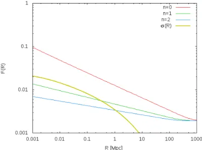
whereσ(R) is the variance in matter fluctuations at a scale R, defined by σ(R) =

Z 1 0

dk

k exp −k²R²

∆²(k), (2.49)

and where ∆(k) is defined by equation (3.14). The normalisation factor of 2, in equation (2.47) is required to account for underdense regions that can exist within overdense regions, this effect is known as the cloud-in-cloud problem, which is not predicted by the original theory. Nevertheless, with the inclusion of this normalisation factor, Numerical simulations have shown that this method to work extremely well [17] and [18]. The value ofδc, is predicted by linear theory to be δc = 1.686, in a flat dark matter-dominated universe.

In section 5.1.1 we will use this formalism to estimate the fraction of the variable chaplygin gas that collapses under the influence of gravity to form structure.

(24)

Chapter 3

Cosmological Observations

In order to evaluate whether a cosmological model is viable, we require a means of comparing its predictions with observational data. As described in section 1.2.3, the CMB is a rich source of information about the state of perturbations in the universe at the last scattering surface. Another observation which is just as important as the CMB is the observed distribution of galaxies. Galaxies are organised in clusters of galaxies which in turn form super-clusters that are separated by large voids. This structure of the universe is often referred to as the cosmic web. Figure 3.1 shows the distribution of galaxies from the Sloan Digital Sky Survey (SDSS) main galaxy redshift sample. The SDSS is an imaging and redshift survey that uses a 2.5 meter wide-angle optical telescope. The SDSS imaging results cover over 35% of the full sky with photometric observations of around 500 million objects and spectra for more than a million objects. The main galaxy sample of this survey is at redshift z ∼0.1 [44].

24

(25)

3.1. THE POWER SPECTRUM 25

Figure 3.1: Large scale structure in the northern equatorial slice of the SDSS main galaxy redshift sample [42]. The slice is 2.5 degrees thick.

This observation is important since this structure must be linked to the initial density fluctuations set up during inflation. Therefore a viable cosmology has to account for, and have the primordial density fluctuations that have evolved to form the large scale structure we observe on large scales today. In this chapter we describe how the theory that describes the evolution of the primordial density fluctuations may be compared with observational data. The subsequent description of the matter and temperature fluctuations will only highlight the important results, assumptions and definitions.

3.1 The Power Spectrum

The previous chapter described the evolution of the primordial density field. To compare theory with observations, i.e., to make quantitative tests of cosmological models, it is necessary to know how to characterise the CMB fluctuations and large scale structure distribution. Cosmological theories are expected to predict the statistical properties of the Universe and not, for example, the exact positions of each overdensity in the dark matter distribution. Therefore, power spectra are very important tools in cosmology, as they can give quantitative information about the variations of a field on different scales. In this section we will study the CMB (temperature fluctuations) and matter power (large scale structure) spectra. We mainly follow the formalism in given in [1, 2].

(26)

26 CHAPTER 3. COSMOLOGICAL OBSERVATIONS

3.1.1 The Matter Power Spectrum

In the case of the large scale structure observations it is useful to take the Fourier transform of the galaxy distribution map in Figure 3.1. The advantage of working in Fourier space is that its easier to distinguish between large and small scales. Work- ing in Fourier space, the most important statistic about the observed large scale structure is the variance in the distribution, known as the matter power spectrum P(k): Consider the Fourier transform of the density fluctuation δ(r),

δ(k) = Z

δ(r)e ^ikrd³r. (3.1)

The power spectrum is then defined as

hδ(k)δ(k⁰)i= (2π)³P(k)δ³(k−k⁰), (3.2) whereδ³ is the Dirac delta function which constrainsk=k⁰.

The construction of the matter power spectrum requires a solution to the evolution of each Fourier modeδ(k, η) and the initial power spectrum generated by inflation.

Performing the Fourier transform effectively means breaking up the function δ(r) into an infinite number of sine waves, each with comoving wavenumber k, and comoving wavelength λ = 2π/k. In conformal time, the density perturbations can be written as

δ(k, η)∝k²T(k)φ(k, η_i)D(η) (3.3) where φ(k, η_i) is the primordial gravitational potential at some initial time η_i and T(k) is known as the transfer function. The transfer function which describes the evolution of the perturbations is a function of scale, while the growth factor D(η) describes the scale independent independent growth at later times. Equation (3.3) together with definition of the power spectrum, equation (3.2), yield

P(k)∝k⁴T²(k)hφ(k, η_i)²iD²(η). (3.4) We relate the potential during this late epoch to the primordial potential, this is achieved through

φ(k, η) = 9

10φ(k, a_i)T(k)D₁(a)

a (3.5)

where the transfer function is defined as

T(k) = φ(k, a_late) φlarge-scale

. (3.6)

This definition is of the transfer function is such that its value is unity on large scales. This is achieved by neglecting the decline in wavelength perturbations as they enter matter-radiation equality. By defining the ratio of the potential to its value at late epochs as

φ(a)

φ(a_late) = D₁(a)

a , (3.7)

(27)

3.1. THE POWER SPECTRUM 27 D₁ becomes the growth of matter perturbations at late times.

Poisson’s equation may be used to relate the matter perturbations and the potential:

φ(k, a) = 4πGρ_ma²δ(k, a)

k² , (3.8)

and recalling how matter evolves with scale factor, ρ_m = Ω_m,0ρ_cr,0/a³ and the definition ρcr,0 = ^3H_8πG⁰², leads to

δ(k, a) = 2 3

k²φ(k, a)a

ΩmH₀² , (3.9)

which may be combined with equation (3.5), to give an expression that relates the overdensity today to the primordial potential:

δ(k, a) = 3 5

k²

ΩmH₀²φ(k, a_i)T(k)D₁(a). (3.10) This equation is independent of how the initial potential φ(k, a_i) was generated, but in the context of inflation, φ(k, a_i) is drawn from a Gaussian distribution with mean variance

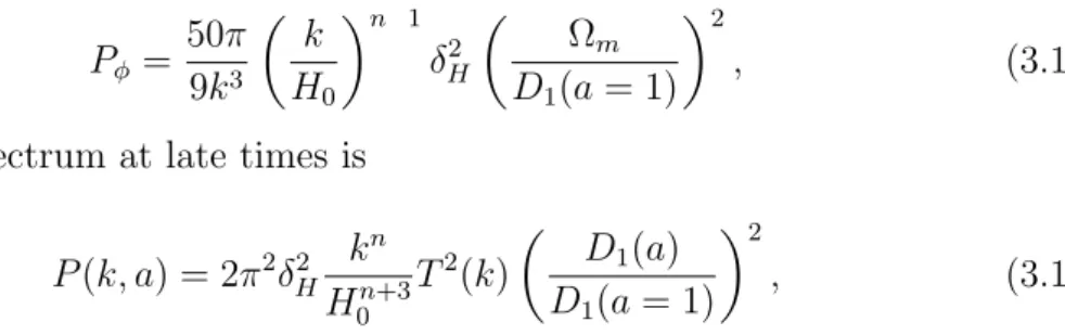
P_φ= 50π 9k³

k H₀

n 1

δ_H²

Ω_m D₁(a= 1)

2

, (3.11)

so the power spectrum at late times is P(k, a) = 2π²δ_H² kⁿ

H₀ⁿ⁺³T²(k)

D₁(a) D₁(a = 1)

2

, (3.12)

where δ²_H is the perturbation amplitude at horizon crossing. The power spectrum has dimensions of (length)³, but to expresses it as a dimensionless quantity, one may associate d³kP(k)/(2π)³ with the excess power in a bin of width k centred at k. Integrating over all orientations of k gives

d³kP(k)/(2π)³ = dk

k ∆²(k), (3.13)

where

∆²(k) = k³P(k)

2π² . (3.14)

Figure 3.2 shows the concordance model matter power spectrum. On large scales the power increases as function of increasing k, then beyond some k_cr the power decreases as function ofk on small scales. To explain this turn-over on small scales, consider that small scales enter the horizon well before matter-radiation equality, i.e., during the radiation epoch, when the potential decays and therefore the transfer function is much smaller than unity. Small scale modes are therefore suppressed from the time they enter the horizon up until the epoch when matter dominates.

Thus the power spectrum is a decreasing function ofk on small scales.

(28)

28 CHAPTER 3. COSMOLOGICAL OBSERVATIONS

10 100 1000 10000 100000

0.0001 0.001 0.01 0.1 1 10

P ( k ) [

Mpc h

3

]

k [hMpc

¹

]

Figure 3.2: Shows the matter power spectrum for the ΛCDM constructed from the WMAP-9 cosmological parameters [45]. This plot was generated using CAMB [49].

3.1.2 The CMB Anisotropy Spectrum

The CMB is observed today as a isotropic radiation field that is very smooth on large scales. However, correcting our relative motion to the CMB rest frame reveals tiny anisotropies in the CMB temperature, of order ∆T /T ∼ 10 5. To first order, these fractional anisotropies only depend on the direction ˆn of the observer. The CMB may be taken to be a 2D-field on the surface of a sphere; one may expand the CMB temperature distribution in spherical harmonics. Therefore the two-point function is a function of multipole moment`, instead of the wavenumberk:

∆T(ˆn)

T =

1

X

`=2

`

X

m= `

a_`mY_`m(ˆn), (3.15)

where thea_`mare the multipole co-efficients and theY_`mare the spherical harmonics.

Each ` corresponds to an angular scale given by θ ≈ 180 /`. Now assuming that the temperature perturbations follow a Gaussian distribution and are statistically isotropic, the powerC_` on angular scales `, may be defined by

ha_`⁰_m⁰a_lmi=C_` δ_`⁰_` δ_m⁰_m. (3.16) The distribution is assumed to Gaussian to ensure that the power spectrum C_` contains all the information, making it the only quantity required to characterise the temperature field. The Kronecker delta’s,δ_i⁰_i, ensure that the power distribution through the multipoles is a function of angular scale. The observed angular power spectrum is given by

C` = 1 2`+ 1

`

X

m= `

|a`m|², (3.17)

(29)

3.1. THE POWER SPECTRUM 29 where C_` is assumed to contain all the statistical information characterising the temperature field, defined by (3.16).

Relating the CMB anisotropies to the density fluctuation, which can be predicted by cosmological models, is the key to extracting the information that was encoded within the CMB temperature field by the cosmic fluid at the last scattering surface.

Assume that the temperature field is given by

T(r,n, η) =ˆ T(η)(1 + Θ(r,n, η)),ˆ (3.18) where Θ is characteristic of the photon perturbation distribution function. The field Θ may be expanded in terms of spherical harmonics [2]:

Θ(r,n, η) =ˆ

1

X

`=1

`

X

m= 1

a`m(r, η)Y`m(ˆn). (3.19) Then using the spherical harmonics othornomality property [2],

Z

dΩY_`m(ˆn)Y_`m0(ˆn) =δ_``⁰δ_mm⁰

, and inverting equation (3.19) by multiplying both sides byY_`m(ˆn) and integrating to obtain

a_`m(r, η) =

Z d³k (2π)³e^{ik r}

Z

dΩY_`m(ˆn)Θ(k,n, η),ˆ (3.20) we may write the angular power spectrum, as defined by equation (3.16), as

C_` =

Z d³k (2π)²

Z

dΩY_`m(ˆn)Θ(k,kˆ·n)ˆ Z

dΩY_`m(ˆn)Θ (k,ˆk·n)ˆ (3.21) where Θ(k,ˆn, η) is the Fourier transform of Θ(r,n, η). Now to obtain an expressionˆ for C_`, one needs hΘ(k,ˆn, η)Θ (k,n, η)i. This expectation value depends on twoˆ separate phenomena: (i) the initial amplitude and the phase of the perturbation is chosen during inflation from a Gaussian distribution and (ii) the evolution of the initial perturbation that turns into anisotropies, i.e., produces the ˆndependence. To simplify, one may write the photon distribution asδ×(Θ/δ), where the dark matter overdensity does not depend on any directional vector. (Θ/δ) does not depend on the initial amplitude, so it can be removed from the averaging over the distribution

hΘ(k,n, η)Θ (k,ˆ n, η)iˆ =hδ(k)δ (k⁰)i

Θ(k,n, η)ˆ δ(k)

Θ (k,n, η)ˆ δ (k)

(3.22) Then, recall the definition of the matter power spectrum ((3.2)). The ratio δ/Θ depends only on the magnitude of k and the dot product ˆk ·ˆn: two modes with the samekand ˆk·nˆ evolve identically regardless of their initial conditions or phase (from now on, the dependence onη may be taken to be implicit). Thus,

hΘ(k,n)Θ (k,ˆ n)iˆ = (2π)³P(k)δ³(k−k⁰) Θ(k,ˆk·n)ˆ δ(k)

! Θ(k,ˆk·n)ˆ δ (k)

!

. (3.23)

(30)

30 CHAPTER 3. COSMOLOGICAL OBSERVATIONS Then combining equation (3.21) with equation (3.23), the angular power spectrum may be related to the density perturbations through

C_` =

Z d³k (2π)²

Z

dΩY_`m(ˆn)Θ(k,ˆk·n)ˆ δ(k)

Z

dΩ⁰Y_`m(ˆn⁰)Θ (k,kˆ·nˆ⁰)

δ(k ) . (3.24) It can be further shown that the angular power spectrum (CMB anisotropies) is related to the matter power spectrum (density fluctuations) through

C_` = 2 π

Z 1 0

dk k²P(k)

Θ_`(k) δ(k)

2

. (3.25)

Generation of CMB Anisotropies

We now present a qualitative description of the mechanism that generates the CMB anisotropies; then we move on to study features of the CMB spectrum.

CMB Anisotropies may be grouped into two categories; primary anisotropies are the anisotropies generated at the last scattering surface and secondary anisotropies are generated along the CMB photon’s path to us. The fluctuations δ_γ already present in the photon density at the surface of last scattering create anisotropies in the CMB. CMB anisotropies are also generated when the CMB photons are gravitationally redshifted or blueshifted by time evolving gravitational potentials.

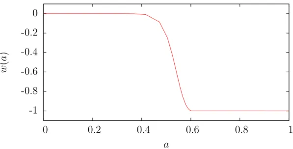
Fluctuations in the matter density will give rise to ‘local’ potential wells (minima) and hills (maxima). Photons lose energy in climbing out of the potential well and are consequently redshifted, while they gain energy when they roll off a potential hill, and are consequently blueshifted. Therefore depending on whether a CMB photon was in potential well or a potential hill at the time of last scattering, its temperature will either be subtly higher or lower. This mechanism of creating temperature fluctuations by variations in the gravitational potential is known as the Sachs-Wolfe effect [43]. The potential wells and hills present at decoupling do not evolve with time as long the universe is matter dominated, and therefore do not generate more anisotropies. However, at a redshift of about z = 0.6 the energy density becomes dominated by dark energy. Then the potential wells and hills are no longer static, these time evolving gravitational potentials generate more temperature fluctuations in the CMB photons. This effect is known as theintegrated Sachs-Wolfe effect (ISW) [43]. Furthermore, bulk velocities of the baryon-photon fluid relative to an observer causes a Doppler shift which also contributes to the CMB anisotropies. To summarise:

∆T

T (ˆn) = 1

4δ_γ+φ(ˆn) + 1

4δ_γ−n·u+ Z η0

lss

dφ

dη (3.26)

where the first term is due to gravitational redshifting by the gravitational potential wells and hills, the Sachs-Wolfe effect. The second term arises from the already existing photon density fluctuations, which are characterised by the Stephen- Boltzmann lawρ_γ=σT⁴ (where σ is the Stephen Boltzmann constant). The third term is due to the relative motion of the baryon-photon fluid with respect to us and

(31)

3.1. THE POWER SPECTRUM 31 the fourth term is due to the ISW effect.

Figure 3.3 shows the CMB anisotropy spectrum, computed using the concordance model with the WMAP-7 best fit cosmological parameters:ΛCDM model; H₀ = 71.0,Ω_c = 0.222,Ω_b,= 0.0449.

100 1000 10000

10 100 1000

C

`(`+1) 2π

` [ µ K

2

]

`

Figure 3.3: Shows ΛCDM CMB Anisotropy spectrum constructed from the WMAP- 9 cosmological parameters[45]. This plot was generated using CAMB [49].

During the period just before the CMB photons were liberated from the baryons cosmic expansion had cooled the CMB photons to a temperature of about T ∼ 3000k. During this epoch, the electrons couple the baryons to the photons by Comp- ton scattering and electromagnetic interactions, resulting a singe baryon-photon fluid. Gravity attracts and compresses the fluid into the potential wells and hills.

Photon pressure counters the compression and sets up acoustic oscillations in the fluid. These acoustic oscillations are frozen into the distribution of photons at recombination. During the radiation domination epoch, the pressure gradients due to the gravitational potentials from matter can be neglected. However, once the gradients have turned infall into acoustic oscillations and the potentials decay, leading to lower amplitudes in the subsequent oscillations.

At the same time the universe continues to cool adiabatically to a point where the photons and baryons decouple. These photons are the CMB photons we de- tect today, which have free streamed from the point of decoupling. Figure 3.3 shows the CMB anisotropy spectrum, this spectrum is computed using thecode for anisotropies in the CMB (CAMB) [49].

In order to study the CMB anisotropy features, we consider a fiducial ΛCDM cosmology constructed from the Wilkinson Microwave Anisotropy Probe (WMAP)- 9yr best fit cosmological parameters [45]. The WMAP is a satellite which measures CMB radiation across the full sky. WMAP measurements play a key role constrain- ing cosmological models, and are well fitted by the current concordance model. In the context of a flat universe, we wish to study the effects of varying some of the ΛCDM cosmological parameters in turn.

(32)

32 CHAPTER 3. COSMOLOGICAL OBSERVATIONS

• Increasing Ω_b,0 increases the amplitudes of the odd peaks over the even peaks, while decreasing Ω_b,0 decreases the amplitudes of the even peaks over the odd ones. This is because baryons drag the baryon-photon fluid deeper into the potential wells. This results in the compressional (odd) peaks being enhanced by the baryons and the rarefaction (even) peaks being suppressed [28].

• Decreasing Ω_c,0 boosts the amplitudes of all the peaks. This predominately affects the higher `, which correspond to the matter-radiation equality epoch, essentially because decreasing Ω_c,0 reduces the matter-radiation ratio.

• Varying Ω_Λ,0 in a flat universe is at the cost of varying Ω_c,0 and visa-versa, so this case is included in the second point.

In ΛCDM, w_Λ(a) = −1. However, since the goal of this thesis is study the effects of a time varying dark energy model we also wish to study the effect of a time varying w on the CMB. Therefore we consider a simple dynamical dark energy model described by the linear relation [53]

wde(a) =α+ (1−a)β (3.27)

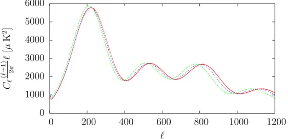
where the constantsα and β are chosen such that −1≤w_de(a)≤0. We then compare the CMB spectra from this model to that obtained from ΛCDM for the same H₀, Ω_b,0 and Ω_c,0. Figure 3.4 shows CMB spectra obtained from the dark energy model defined by Equation (3.27) for {α, β} = {−1,0.9},{−1,0.5} (green,blue) and the red curve is the ΛCDM spectrum. These plots are for the same cosmological parameters except that they have different equation of state parameters. For the model with β = 0.5, the equation of state parameter deviates from −1 at an earlier time, i.e., the model tends towards ΛCDM later than the β = 0.9 model.

We see that a time varying dark energy component shifts the position of the peaks to smaller `, which enhances the amplitudes of the first peaks. This effect is more evident in the model with β = 0.5. This shift in amplitude peaks is a result of a smaller distance to the scattering surface caused by the time evolving w(a). This is because the point of last scattering occurs at a lower redshift for dynamical DE models since there is higher ρ_de at early times at the expense of ρ_c (flat universe) which delays matter-radiation equality and subsequently the point of decoupling.

To illustrate, consider a dark energy model which has w(a) > −1 at some early time t_i. According to equation (1.9) this model will have higher density at time t_i compared to a model with w=−1.

(33)

3.2. THE LIKELIHOOD FUNCTION 33

0 1000 2000 3000 4000 5000 6000

0 200 400 600 800 1000 1200

C`(`+1) 2π`[µK2 ]

`

Figure 3.4: Shows the CMB spectra for the for two dynamical dark energy models described by Equation (3.27), with {α, β} ={−1,0.9},{−1,0.5} (green,blue) and the red curve is the ΛCDM model same set of parameters except thatw(a) is varying the dynamical DE models. This plot was generated using CAMB [49].

3.2 The Likelihood Function

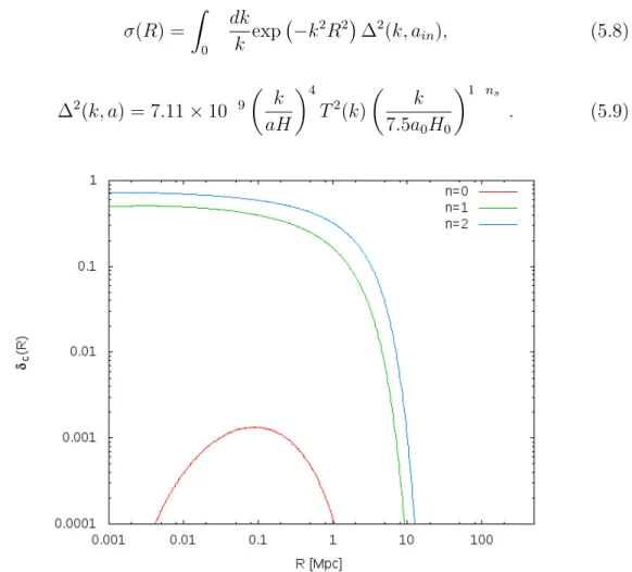
The evaluation of cosmological models in light of observational data is key in both theoretical and observational cosmology. Recent analysis is based on the likelihood function, which is a function of the param