UNIVERSITY OF KWAZULU-NATAL
Link Adaptation for Quadrature Spatial Modulation
Segun Emmanuel Oladoyinbo
2016
i
Link Adaptation for Quadrature Spatial Modulation
By Segun Emmanuel Oladoyinbo Student Number: 214574841
Submitted in fulfilment of the academic requirements of Master of Science in Engineering
School of Engineering
College of Agriculture, Engineering and Science University of KwaZulu-Natal
Howard College South Africa
Supervised by: Dr Narushan Pillay Co-supervised by: Prof HongJun Xu
July 2016
ii
CERTIFICATION
As the candidate’s Supervisor I agree to the submission of this dissertation.
___________________________
Signed: Dr Narushan Pillay Date: 28th July, 2016
iii
DECLARATION 1 - PLAGIARISM
I, Segun Emmanuel Oladoyinbo declare that:
1. The research reported in this dissertation, except where otherwise indicated, is my original research.
2. This dissertation has not been submitted for any degree or examination at any other university.
3. This dissertation does not contain other persons’ data, pictures, graphs or other information, unless specifically acknowledged as being sourced from other persons.
4. This dissertation does not contain other persons' writing, unless specifically acknowledged as being sourced from other researchers. Where other written sources have been quoted, then:
a. Their words have been re-written but the general information attributed to them has been referenced
b. Where their exact words have been used, then their writing has been placed in italics and inside quotation marks, and referenced.
5. This dissertation does not contain texts, graphics or tables copied and pasted from the internet, unless specifically acknowledged, and the source being detailed in the thesis and in the Reference section.
_____________________
Signed: Oladoyinbo Segun Date: 28th July, 2016
iv
DECLARATION 2 - PUBLICATIONS
The work in this dissertation will be submitted to IET communications journal for publication.
The detail is as follows:
S. Oladoyinbo, N. Pillay, H. Xu “Adaptive quadrature spatial modulation,” [Ready for submission to IET Communications Journal].
_____________________
Signed: Oladoyinbo Segun Date: 28th July, 2016
v
ACKNOWLEDGEMENTS
I want to give all the glory to God for the gift of life and the strength granted onto me in the course of this research and for making it a possibility “…but with God all things are possible, Matthew 19:26 ”.
My gratitude goes to my supervisors, Dr Narushan Pillay and Prof H. Xu, for your time, encouragement, training as a researcher from wealth of experience, guidance and unlimited access to your office anytime I come around for help during this period. To my family members, I say a big thank you. My parents: Elder. P.O Oladoyinbo and Mrs W.A Oladoyinbo deserve a bigger thank you for their encouragement, may you live long to enjoy the fruit of your labour in Jesus name. Desire (Ajike mi), Ayobami, Ife, Olayide (Aduke temi ni kan), Ashaolus’
and Seun Oyebode are not left out. Finally, to my loved ones, brothers, friends and well- wishers, thank you all for your supports, motivations and prayers. Gracias
vi
DEDICATION
This dissertation is dedicated to my lovely wife, Olayide Adebimpe and my beautiful daughter Desire Lois.
vii
ABSTRACT
Quadrature spatial modulation (QSM) maintains all of the advantages of spatial modulation but further improves upon its spectral efficiency by the logarithm base two of the number of transmit antennas. However, further improvement in terms of reliability can still be achieved.
On this note, in this dissertation, link adaptation for QSM is investigated.
The existing analytical error performance for QSM does not agree well with Monte Carlo simulation results in the low signal-to-noise ratio (SNR) region. Therefore, the first contribution is a lower bound approach to the analytical error performance, which agrees well with simulation results for low to high SNRs.
Secondly, link adaptation is investigated on conventional QSM system to further improve upon the reliability of the system (QSM). Assuming a slowly varying channel and full knowledge thereof, the proposed scheme is based on employing unique candidate transmission modes, chosen to satisfy a target spectral efficiency. The proposed scheme employs optimal transmit antenna selection and constellation selection so as to minimize the instantaneous bit error probability (IBEP). The candidate mode with the minimum IBEP is activated for transmission.
Significant SNR gain is demonstrated by the proposed scheme over QSM.
Finally, the effects of low-complexity transmit antenna selection for AQSM scheme is investigated to further reduce the computational complexity (CC) overhead. The selection is based on computing the channel amplitude and antenna correlation to eliminate the poor channel(s). Monte Carlo simulation results demonstrate a trade-off between CC and reliability in comparison to the use of optimal antenna selection.
viii
TABLE OF CONTENTS
CERTIFICATION ... ii
ACKNOWLEDGEMENTS ... v
DEDICATION ... vi
ABSTRACT ... vii
TABLE OF CONTENTS ... viii
LIST OF FIGURES ... xii
LIST OF TABLES ... xiii
LIST OF ACRONYMS ... xiv
CHAPTER 1 ... 1
INTRODUCTION ... 1
1 Multiple-Input Multiple-Output ... 1
1.1 Categories and Techniques of MIMO ... 1
1.2 System Model for a MIMO System ... 2
1.3 Innovative Forms of MIMO ... 4
1.3.1 Vertical-Bell Laboratories Layered Space-Time Architecture ... 5
1.3.2 The Alamouti Space-Time Block Code ... 5
1.3.3 Spatial Modulation ... 5
1.3.3.1 Features of Spatial Modulation ... 6
1.3.3.2 Improvement Achieved in SM in Terms of Error Performance and CC ... 6
1.3.3.3 Transmit Antenna Selection for SM... 6
1.3.3.4 Generalized Spatial Modulation ... 8
1.3.3.5 Link Adaptation ... 8
ix
1.3.3.6 Improved Spectral Efficiency for SM ... 10
1.4 Research Motivation and Problem Statement ... 10
1.5 Research Objectives ... 12
1.6 Organisation of Dissertation ... 12
1.7 Major Contribution of the Research ... 12
1.7.1 Study and Performance Analysis of QSM ... 12
1.7.2 Link Adaptation for QSM ... 13
1.8 Notation used in the Dissertation ... 13
CHAPTER 2 ... 14
2 Introduction ... 14
2.1 Transmission Model of Spatial Modulation ... 14
2.1.1 Optimal Detection for Spatial Modulation ... 16
2.2 Performance Analysis for Spatial Modulation ... 17
2.2.1 Analysis of Symbol Estimation ... 18
2.2.2 Analysis of Transmit Antenna Index Estimation ... 18
2.3 Numerical Analysis of the Computed Analytical and Simulated BER for Spatial Modulation ... 19
2.4 Chapter Summary ... 22
CHAPTER 3 ... 23
Quadrature Spatial Modulation ... 23
3 Introduction ... 23
3.1 System Model of Quadrature Spatial Modulation ... 24
3.1.1 Optimal Detection ... 27
x
3.2 Performance Analysis of M-QAM Quadrature Spatial Modulation using Asymptotic
Tight Union Bound ... 27
3.3 The Proposed Performance Analysis for M-QAM Quadrature Spatial Modulation ... 29
3.3.1 Analytical Average BER of Symbol Estimation ... 30
3.3.2 Analytical Average BER of Transmit Antenna Index Estimation ... 30
3.4 Numerical Analysis of the Computed Analytical BER and Simulated BER for Quadrature Spatial Modulation ... 31
3.5 Chapter Summary ... 35
CHAPTER 4 ... 36
Adaptive Quadrature Spatial Modulation ... 36
4 Introduction ... 36
4.1 System Model for the Proposed Adaptive Quadrature Spatial Modulation ... 38
4.2 Analysis of Instantaneous Bit Error Probability for Adaptive Quadrature Spatial Modulation ... 39
4.2.1 Analysis of Symbol Estimation Employing a Single Transmit Antenna ... 40
4.2.2 Analysis of Symbol Estimation Employing Two Transmit Antennas ... 40
4.2.3 Analysis of Transmit Antenna Index Estimation Employing a Single Transmit Antenna ………..41
4.2.4 Analysis of Transmit Antenna Index Estimation Employing Two Transmit Antennas. ... 43
4.3 The Proposed AQSM System Based on Euclidean Distance Antenna Selection ... 44
4.3.1 Background ... 44
4.3.2 Algorithm 1 ... 46
xi
4.4 The Proposed AQSM System with Antenna Selection Based on Channel Amplitude
and Antenna Correlation ... 49
4.4.1 Algorithm 2 ... 49
4.5 Computational Complexity Analysis for the Proposed Topology ... 53
4.5.1 Computational Complexity Analysis for Transmit Antenna Selection based on EDAS ………..53
4.5.2 Computational Complexity Analysis for Transmit Antenna Selection based on Channel Amplitude and Antenna Correlation ... 54
4.5.3 Computational Complexity Analysis for the Proposed Topology Based on EDAS ………..54
4.5.4 Computational Complexity Analysis for the Proposed Topology Based on Channel Amplitude and Antenna Correlation ... 55
4.6 Numerical Analysis of the BER Performance for Adaptive Quadrature Spatial Modulation ... 56
4.7 Chapter Summary ... 59
CHAPTER 5 ... 60
Conclusion and Future Work ... 60
5 Conclusion ... 60
5.1 Future Work ... 62
REFERENCE………..…….63
xii
LIST OF FIGURES
Figure 1-1 System Model for a MIMO system ... 2
Figure 1-2 System model for low-complexity Euclidean distance transmit antenna selection. .... 7
Figure 2-1 System model for Spatial Modulation. ... 14
Figure 2-2 Validation of 4-QAM 2 × 4 and 2 × 2 SM theoretical analysis with the Monte Carlo simulation result ... 20
Figure 2-3 Validation of 16-QAM 2 × 4 and 2 × 2 SM theoretical analysis with the Monte Carlo simulation result ... 21
Figure 2-4 Validation of 64-QAM 4 × 4 and 4 × 2 SM theoretical analysis with the Monte Carlo simulation result ... 22
Figure 3-1 System model for quadrature spatial modulation ... 24
Figure 3-2 16-QAM constellation points ... 26
Figure 3-3 BER performance of QSM for 4 b/s/Hz. ... 32
Figure 3-4 BER performance of QSM for 6 b/s/Hz. ... 33
Figure 3-5 BER performance of QSM for 8 b/s/Hz ... 34
Figure 4-1 System model of the proposed AQSM ... 38
Figure 4-2 Comparison of BER performance between AQSM, AQSM-EDAS and QSM for 6 b/s/Hz considering NR= 2. ... 57
Figure 4-3 Comparison of BER performance between AQSM, AQSM-EDAS and QSM for 8 b/s/Hz considering NR= 2. ... 58
xiii
LIST OF TABLES
Table 2-1 Gray-coded constellation points for 4-QAM modulation order. ... 15
Table 2-2 Mapping process for 2 × 4 4-QAM SM system. ... 15
Table 3-1 Mapping process of QSM system. ... 25
Table 3-2 SNR gain (dB) of QSM achieved over SM ... 35
Table 3-3 SNR gain (dB) variation of lower bound approach achieved over asymptotic union bound ... 35
Table 4-1 Numerical Comparison of Computational Complexity of EDAS and LCTAS-A-C .. 54
Table 4-2 Numerical Comparison of Computational Complexity of EDAS-AQSM and LCTAS- A-C-AQSM ... 56
Table 5-1 SNR gain (dB) of AQSM as compared to QSM and SM at a BER of 10-5 ... 61
Table 5-2 Numerical comparison of Computational Complexity of AQSM-EDAS and AQSM- LCTAS ... 61
xiv
LIST OF ACRONYMS
APM………..Amplitude/Phase Modulation AQSM………Adaptive Quadrature Spatial Modulation AQSM-EDAS………Adaptive Quadrature Spatial Modulation based on EDAS AQSM-LCTAS………Adaptive Quadrature Spatial Modulation based on LCTAS ASM………..Adaptive Spatial Modulation AWGN ………..Additive White Gaussian Noise BER………Bit Error Rate BPSK……….Binary Phase Shift Keying CC……….Computational Complexity CSI……….Channel State Information EDAS………..Euclidean Distance Antenna Selection FRFC………...Frequency-Flat Rayleigh Fading channel GSM………..Generalized Spatial Modulation i.i.d. ……….Independent and Identically Distributed IAS………..Inter-Antenna Synchronization IBEP……….Instantaneous Bit Error Probability ICI………..Inter-Channel Interference IEEE………..Institute of Electrical and Electronic Engineers ISI………Inter-Symbol Interference LCTAS………Low-Complexity Transmit Antenna Selection LCTAS-A-C………LCTAS based on Channel Amplitude and Antenna Correlation MA-GSM………Multiple Active Transmit Antenna for Generalized Spatial Modulation MGF………..Moment Generating Function MIMO………Multiple-Input Multiple-Output ML……….Maximum Likelihood PDF………Probability Density Function PEP……….Pairwise Error Probability PSK………Phase Shift Keying QAM………Quadrature Amplitude Modulation QPSK……….Quadrature Phase Shift Keying QSM………Quadrature Spatial Modulation RF………..Radio Frequency SER………Symbol Error Rate SM………..Spatial Modulation
xv
SM-OD………Spatial Modulation with Optimal Detection SMUX………..Spatial Multiplexing SNR………...Signal-to-Noise Ratio STBC……….Space-Time Block Code SVD……….Signal Vector Based Detection TAS………..Transmit Antenna Selection V-BLAST………Vertical Bell Laboratories Layered Space-Time Architecture
1
CHAPTER 1 INTRODUCTION 1 Multiple-Input Multiple-Output
Multiple-input multiple-output (MIMO) systems have shown tremendous promise over the years with regards to its high transmission capacity and superior system reliability in a wireless communication scenario [1]. Traditionally, the data to be transmitted in MIMO systems is encoded and divided into parallel data streams, each of which is modulated by a separate transmitter. During transmission, the data streams are captured by multiple antennas, which are slightly different in phase, each antenna can be treated as a separate channel in MIMO systems.
The antenna takes advantage of the multiple channels to transfer data, thus, increasing throughput [2]. The data rate per channel increases linearly with the number of different data streams that are transmitted in the same channel, providing scalability and a more reliable link.
MIMO systems have the benefit of increase in capacity, transmission range and robustness, such that it permits multiple data streams. In addition, it helps to improve the signal-to-noise ratio (SNR) and reliability significantly. However, due to the simultaneous transmission of data in MIMO systems, inter-antenna synchronization (IAS) is required at the transmitter and inter- channel interference (ICI) is experienced at the receiver [1, 3].
1.1 Categories and Techniques of MIMO
In [4], MIMO systems are categorized according to their transmission techniques, which can be divided into three main categories. These are as follows:
1. Spatial multiplexing: Signals are split into bit streams and each stream is transmitted from a different transmit antenna in the same frequency channel. If the signals arrive at the receiver with highly different spatial signatures and accurate channel state information (CSI), the receiver can separate the bit stream into a perfect parallel channel. The maximum number of streams that the signal can be split into is limited by the number of available transmit antennas [1, 3]. Similarly, the assumption of known CSI in spatial multiplexing can be used with precoding [5]. Spatial multiplexing can be employed for simultaneous transmission to multiple receivers (space division multiple access) [6], which requires the knowledge of the CSI at the transmitter as good separability is achieved with scheduling receivers.
2
2. Diversity coding: The term ‘diversity’ has been given different meanings over time in wireless communication scenarios. The variation of the channel in time, frequency and space with multiple copies of data arriving at the receiver can be defined as diversity.
The amount of improvement that can be achieved in terms of the received signal (in diversity scheme) depends on the fading characteristics of the transmitted signal. This technique exploits the independent fading in the channel to enhance the reliability of the system. In diversity coding, the knowledge of the CSI is not needed at the transmitter as a single stream of data is transmitted; but the transmitted signal is coded with a technique called space-time coding prior to transmission [4].
3. Precoding: This is a type of transmit diversity technique which sends out pre-coded information to the receiver according to the known CSI, employing multi- stream beamforming. The signal is transmitted from each of the available transmit antennas with the appropriate phase and amplitude in order to maximize the SNR and transmitting power. Precoding techniques have the benefit of summing up the transmitted signals from different antennas, constructively at the receiver. Thus, increasing the signal gain at the receiver and reducing fading effects. However, knowledge of the CSI is required at the transmitter for precoding, to assist in maximizing the signal level at the receiver [4].
1.2 System Model for a MIMO System
Figure 1-1 System Model for a MIMO system [7]
T ra n s m itt e r . . .
Transmitted signal vector
Received signal vector 1
2
R e c e iv e r
. . .
1
2
N
Rn
1n
2NR
n
NT
h
1,1h
2,1,
R NT
h
N3
Figure 1-1 illustrates a typical MIMO system with 𝑁𝑇 transmit antennas and 𝑁𝑅 receive antennas with multipath fading channel 𝑯 between the transmitter and the receiver. The respective path of the channel 𝑯 used for transmission with a constant channel gain can be represented as:
𝑯 = [𝒉1 𝒉2 𝒉3 … 𝒉𝑁𝑇]𝑇 (1-1)
The channel matrix between the transmit antennas 𝑁𝑇 and receive antennas 𝑁𝑅 with dimension 𝑁𝑅× 𝑁𝑇 can be expressed as:
𝑯 = [
ℎ1,1 ⋯ ℎ1,𝑁𝑇
⋮ ⋱ ⋮
ℎ𝑁𝑅,1 ⋯ ℎ𝑁𝑅,𝑁𝑇] (1-2)
where ℎ𝑖,𝑗 is the corresponding row and column of the channel 𝑯, respectively, used for transmission at a particular time 𝑡, i. e. 𝑖 ∈ [1: 𝑁𝑅] and 𝑗 ∈ [1: 𝑁𝑇].
Wireless channels are categorized into large-scale fading and small-scale fading [8].
1. Large-scale fading is distance dependant, as signal power decreases over time due to path loss of the transmitted signal and foliage in the signal path.
2. Small-scale fading occurs due to multipath of the channel resulting to the distortion of the signal in amplitude, phase and angle of arrival. It is caused by multipath of the signal propagation.
In this dissertation, a frequency-flat Rayleigh fading channel is used. This is mostly seen in an environment with high environmental propagation effect on the radio wave or where line of sight (LOS) is absent. Especially, in the urban areas where there are large number of reflectors.
A signal 𝒙 of dimension 𝑁𝑇× 1, i.e. 𝒙 = [𝑥1 𝑥2 𝑥3… 𝑥𝑁𝑇]𝑇is transmitted over the MIMO multipath fading channel 𝑯 as shown in the Figure 1-1. This is considered in the presence of additive white Gaussian noise (AWGN) represented by a vector 𝒏 of dimension 𝑁𝑅× 1, i.e.
4
𝒏 = [𝑛1 𝑛2 𝑛3… 𝑛𝑁𝑅]𝑇 with Gaussian distribution 𝐶𝑁 (0,1) and with independent and identically distributed (i.i.d) entries. Then, the received signal 𝒚 becomes:
𝒚 = √𝜌 𝑯𝒙 + 𝒏 (1-3)
where 𝜌 is the average SNR.
Note, the channel used is a frequency-flat Rayleigh multipath fading channel between the transmitter and the receiver, such that the bandwidth of the signal 𝒙 is less than the coherence bandwidth of the channel 𝑯 resulting in a constant channel gain over the transmitted signal bandwidth.
Despite the advantages of MIMO systems, it still has some limitations such as the need for IAS at the transmitter due to the simultaneous transmission of data, high power consumption considering all the antennas are active at the same time and ICI is experienced at the receiver considering all transmit antennas are transmitting at the same time.
In the next sub-section, techniques used to improve the limitations of conventional MIMO systems will be discussed and examples of MIMO systems including innovative forms of MIMO will be presented in Section 1.3.
1.3 Innovative Forms of MIMO
Spatial multiplexing is a suitable scheme for future wireless communication due to the high demand for capacity in multimedia services. However, coupling of symbols in time and space in spatial multiplexing causes high ICI and simultaneous transmission of data requires IAS at the transmitter [8]. These are the major limitations of spatial multiplexing. The reliability of the MIMO system is key, in which spatial diversity plays a major role. However, spatial diversity techniques have a major limitation of ISI due to the dispersion of the channel. This can be avoided if enough space is left between the transmitted symbols. Although, this will cause decreased throughput [9, 10]. Various examples of innovative systems, employing spatial multiplexing and spatial diversity will be discussed in the next sub-section, starting with a prominent example of MIMO system, the Vertical-Bell Laboratories Layered Space-Time Architecture (V-BLAST) [11].
5
1.3.1 Vertical-Bell Laboratories Layered Space-Time Architecture
V-BLAST employs spatial multiplexing to increase the spectral efficiency of the system by sending out 𝑁𝑇 (total number of the available transmit antennas) signals at each time slot. This results to increase throughput by dividing the input bit stream into sub-streams and transmitting it in parallel through a specific antenna. However, ICI and IAS exists in V-BLAST technology, since all transmit antennas transmit data streams simultaneously [11].
In an indoor environment a spectral efficiency of 20 b/s/Hz can be achieved in V-BLAST technology assuming a practical SNR range [11]. In addition, a block of 𝑁𝑇 symbols is compressed into a single symbol prior to transmission, so that an algorithm that maps the symbol to just one of the 𝑁𝑇 can be employed to retain the information, ICI experienced at the receiver can be avoided [12].
1.3.2 The Alamouti Space-Time Block Code
The Alamouti Space-Time Block Code (STBC) [13], is an example of an improved MIMO system. The Alamouti STBC exploits spatial diversity to improve the reliability of the system by sending two symbols in its first time slot such as 𝑥1 and 𝑥2. The negative conjugate of the second symbol sent in the first time slot, i.e. (−𝑥2∗) together with the conjugate of the first symbol, i.e. (𝑥1∗) is sent during the second time slot such that, the transmitted signal 𝑿 = [ 𝑥1 𝑥2
−𝑥2∗ 𝑥1∗].
Since, this still requires two time slots to send out two symbols, the data rate remains the same [13, 14]. But, the reliability of the link has improved due to the redundant copies of data transmitted to the receiver over an independent channel. However, in the Alamouti STBC, the computational complexity (CC) at the receiver increases exponentially with the size of the constellation, which makes the implementation not only difficult but expensive [13].
1.3.3 Spatial Modulation
Spatial Modulation (SM) [15-17], is another innovative form of MIMO system proposed by Mesleh et al.. SM eliminates the major limitations of IAS and ICI experienced in conventional MIMO by employing multiple transmit antennas in an innovative manner. This is made possible by using a dimension called the spatial (antenna) dimension to convey additional information.
In SM, only one transmit antenna is active at each transmission instant, eliminating the need for IAS at the transmitter and ICI at the receiver. Additionally, SM uses the space modulation technique to enhance the error performance and capacity of the system [16]. The Monte Carlo
6
simulation results for SM demonstrates significant improvement in terms of error performance over V-BLAST [15].
1.3.3.1 Features of Spatial Modulation The main features of SM are listed below:
1. Single RF chain is used to make the system more cost effective and energy efficient [16].
2. ICI and IAS are totally avoided in SM [16].
3. High spectral efficiency is achieved in SM [15, 16].
The benefits of SM, which includes: reduction in hardware cost, high energy efficiency, elimination of major limitations experienced in conventional MIMO system and increase in throughput with improved error performance, makes SM one of the most promising MIMO systems.
Despite the advantages, SM still has few limitations such as:
1. It requires transmit antennas in the power of two.
2. Its data rate enhancement increases only in logarithm base-two of the total number of transmit antennas compared to other spatial multiplexing techniques.
3. Transmit diversity was not exploited in SM
Due to clear advantages of SM, we present a detailed survey of the primary works of SM. In the next sub-section, improvement achieved in SM in terms of error performance, CC and spectral efficiency will be discussed.
1.3.3.2 Improvement Achieved in SM in Terms of Error Performance and CC
Application of transmit diversity and receive diversity or a combination of both in MIMO systems allow huge improvement to be achieved in terms of error performance [18].
Furthermore, introducing transmit antenna selection (TAS) into a system can further improve its error performance [18].
1.3.3.3 Transmit Antenna Selection for SM
The demand for high data rates in multimedia services, which requires scheme with improved error performance coupled with very high spectral efficiency. This will in turn increase the CC of the system as the spectral efficiency increases, due to the increase in the number of required transmit antennas [18]. TAS has been beneficial in SM system, as it further reduces hardware complexity and cost, achieving diversity gain.
7
Figure 1-2 System model for low-complexity Euclidean distance transmit antenna selection [19].
The application of TAS, a transmit diversity technique is used in SM system to achieve considerable improvement in error performance. For instance, Euclidean distance based antenna selection (EDAS) was investigated in SM [20, 21], taking advantage of the ICI and IAS free property of SM and separating the QAM signal sets to further improve the error performance of the system. However, a further reduced CC version of this approach was proposed by Rajashekar et al. and investigated in [22], employing the approach of only one search across symmetrical constellation sets making SM practically implementable.
Recently, researchers announced the new achievement made in low-complexity transmit antenna selection (LCTAS). In [23], a low-complexity technique for both detection and antenna selection for SM was presented, employing maximum gain transmit antenna selection (MG- TAS) to reduce the average energy consumption in the system by calculating the channel gains and choosing the channel with the minimum gain for transmission.
In [19], a LCTAS was proposed by Pillay et al., where channel amplitude and antenna correlation are used to select the best channel prior to transmission. The scheme exhibits a very low CC when compared to EDAS-SM. Hence, this yields a highly realizable MIMO scheme with reduced CC, making SM more realizable. An algorithm based on both schemes will be further explained/discussed in Chapter 4 of this dissertation.
SM Transmitter
SM Receiver
H
Antenna Selection
Channel state information
Feedback Link
1 1
2 2
. . . . . .
NT NR
8 1.3.3.4 Generalized Spatial Modulation
In addition, a multiple active transmit antenna scheme for generalized spatial modulation (MA- GSM) was proposed in [24] to reduce the CC of the novel GSM system which requires a high number of transmit antennas to achieve high data rate. The proposed MA-GSM uses multiple transmit antennas to convey different information at each time slot similar to the conventional SM system. Significant improvement was achieved in terms of CC in the proposed system as 10 b/s/Hz, QPSK system which requires 8 transmits antennas in conventional GSM system and 64 antennas in SM system requires only 4 transmit antennas in MA-GSM system, thus, improving the high CC with respect to high data rate.
1.3.3.5 Link Adaptation
To construct schemes with full-rate, full-diversity with spatial multiplexing such as V-BLAST, which can give high multiplexing gain for more than two transmit antennas with linear CC is impossible [24]. Likewise, It has been stated in literature that link adaptation can improve the reliability of a MIMO system [25, 26].
The process of adapting the error correction with the modulation scheme according to the condition of the link at that instant to achieve high efficiency in the system is called link adaptation [27]. Such that with a very good link, a highly efficient modulation scheme is employed and vice versa.
1.3.3.5.1 Adaptive Spatial Modulation
Adaptive SM (ASM) was investigated in [26], with maximum-likelihood (ML) based detector, which searches over the entire signal space to obtain better system performance using the CSI estimated by the receiver as a decision metric to select the optimum candidate for transmission.
Likewise, link adaptation for SM was investigated in [28], using power allocation algorithm by shrinking the error vector space and exploiting only the Euclidean distance of the dominant error vectors to optimize the power allocation matrix solving the effect of power imbalance stated in [29].
Another approach of link adaptation was investigated in [30], using pre-processing pre-coder formulation technique at the transmitter prior to transmission to achieve transmit diversity. This is done by maximizing the minimum Euclidean distance among the pre-coded codewords. Thus, improving the error performance of the system with reduced CC.
A similar approach to [30] was proposed in [31], employing two different transmit pre-coding algorithm. One is based on maximizing the minimum Euclidean distance between the SM
9
constellation points at the receiver as against among the codewords in [30]. The second algorithm in [31] is based on minimizing the bit error rate (BER) of SM which can jointly maximize the overall Euclidean distance between the received signal points. The Monte Carlo simulation results show that the second algorithm proposed in [31] (using minimum BER) achieved significant improvement when compared to the first algorithm (maximizing the minimum Euclidean distance) and power allocation algorithm stated earlier [28].
However, in [26], an approach similar to [31] was employed to improve the error performance using a CSI estimated by the receiver as a decision metric to select the mode with the least bit error rate (BER) as the transmitting mode. Different transmission candidate modes with the same target spectral efficiency coupled with LCTAS was employed.
The combination of two transmit diversity schemes link adaptation and TAS was employed in [26] to decrease the extreme high CC in [25]. This employs different transmission candidate modes with the same target spectral efficiency. The decision metric in [25, 26], is based on selecting the transmission candidate mode that maximizes the minimum Euclidean distance as the transmission mode at that instant.
In all the techniques discussed so far, significant improvement was achieved either in error performance or reduction in CC and at times with increased data rate. The CC in the decision metric in [25] was reduced in [26]. Similarly, in [31], the CC imposed on the system can be further reduced by employing a decision metric, which can adopt a lookup table (LUT) computation technique [32].
In this dissertation, we proposed a low CC decision metric, to achieve a lower CC in the system, computing the instantaneous bit error probability (IBEP) and the transmission candidate mode with the minimum IBEP is selected as the transmission mode. Capitalizing on the LUT computation technique and assuming the full knowledge of the channel is known at the receiver.
Likewise, a sub-optimal transmit antenna selection proposed in [19, 23] is employed to further reduce the CC by evaluating the channel amplitude and antenna correlation to eliminate the worse channel at that instant. We aim at maximizing the advantage of free ICI and IAS in the system and decreasing the CC in joint detection at the receiver. This will be discussed in details in Chapter 4 in this dissertation.
The second limitation of SM mentioned in Section 1.3.3.1, of its data rate enhancement being proportional to logarithm base-two of the total transmit antennas unlike other spatial multiplexing techniques, such as V-BLAST, whose data rate increases linearly with the number
10
of transmit antennas was improved on by further decomposing the spatial dimension into in- phase and quadrature-phase components [33].
This brought about an enhanced spectral efficiency form of SM called quadrature spatial modulation (QSM) [33, 34]. This will be further discussed in next sub-section and Chapter 3 of this dissertation.
1.3.3.6 Improved Spectral Efficiency for SM
QSM, an SM-based scheme, uses transmit antennas in an innovative manner to enhance the performance and throughput of the conventional SM system by using an extra spatial dimension called the quadrature-phase dimension. The spatial constellation of QSM is extended into in- phase and quadrature-phase dimensions. In QSM, the first dimension (in-phase) transmits the real part of the decomposed constellation symbol, while the second dimension (quadrature- phase) transmits the imaginary part.
In the same way, ICI and IAS are avoided completely in QSM due to symbols being orthogonal and modulated into the cosine and sine carriers, respectively [33]. This approach improves the criticism of SM by using an additional logarithm base two of the total transmit antennas.
Significant improvement was achieved in QSM when compared to a conventional SM system of the same spectral efficiency [33, 34]. This will be more elaborated on in Chapter 3 of this dissertation.
1.4 Research Motivation and Problem Statement
MIMO systems have been investigated in numerous papers as the future of wireless communication scenario [1]. Recent studies have led to the development of an innovative scheme of MIMO systems called SM [15], which employs the spatial dimension to convey additional information and requires only a single RF chain for transmission, avoiding IAS and ICI completely.
The criticism of SM, of its data rate enhancement increasing only in logarithm base-two of the total number of transmit antennas compared to other spatial multiplexing techniques, brought about an enhanced spectral efficiency of SM called QSM.
QSM proposed in [33, 34], extends the spatial constellation dimension to the in-phase and quadrature-phase dimensions, which are modulated into the cosine and sine carriers, respectively, to eliminate IAS and ICI completely. QSM improves the spectral efficiency of SM by considering the additional spatial dimension (quadrature-phase) to convey information.
11
Significant improvement in terms of data rate was achieved in QSM when compared to a conventional SM system [33].
In [33], the overall bit error probability of QSM was derived using an asymptotic tight union bound, which does not match at the low SNR region. In [7], the overall bit error probability of SM was derived using a lower bound approach. Result shows that the approach in [7] matches very closely at lower SNR validating the results from low SNR to high SNR region than the approach employed in [33], which employs an asymptotic tight union bound. This motivates for the formulation of the theoretical analysis of QSM using a lower bound approach to validate the Monte Carlo simulation results.
The similarity and attractive features of SM and QSM include avoidance of ICI and IAS, which formed the major limitation of conventional MIMO systems. QSM exhibits significant improvement when compared to a conventional SM of the same spectral efficiency [15, 33]. In addition, link adaptation has been stated in literature that, it can further improve the error performance of a MIMO system. As investigated in [25, 26, 35], which demonstrates that link adaptation in MIMO system can further improve the error performance of the system.
In this dissertation, we propose an algorithm that employs different candidate transmission mode depending on the condition of the transmission link, such that with a very good link a highly efficient modulation scheme is employed and vice versa. The proposed scheme is called adaptive quadrature spatial modulation (AQSM).
Similarly, incorporating an optimal TAS investigated in [22] to the proposed system to further improve the error performance, imposed a high CC to the system. However, LCTAS as proposed by Pillay et al. [19], employing a metric of the larger the amplitude of the channel the better it is and discarding the transmit antenna based on high correlation to reduce the CC in the joint detection at the receiver. Thereby, computing the channel amplitude and antenna correlation prior to transmission to eliminate the worse channel at each transmission instant.
The CC of the TAS proposed in [22] is high compared to the technique proposed in [19]. This demonstrates a very low CC as shown in the CC analysis in [19].
The decision metric in the link adaptation technique employed in [25] impose a very high CC in the system as compared to the decision metric employed in [26]. However, the CC in the decision metric in [26] and [31] can be reduced employing LCTAS using channel amplitude and antenna correlation [19]. This can be combined with link adaptation technique using a similar approach to [26], but with a decision metric of the minimum IBEP to select the transmission mode. Capitalizing on the LUT computation technique that can be adopted, this motivates the application of link adaptation in QSM system.
12
1.5 Research Objectives
The following are the objectives of this research:
1. Formulation of the average bit error probability for QSM system using a lower bound approach, which gives a better match across the SNR range.
2. Formulation of AQSM in terms of IBEP using a lower bound approach.
3. Investigation of an optimal TAS in the proposed AQSM system.
4. Investigation of LCTAS in the proposed AQSM system.
1.6 Organisation of Dissertation
The rest of the dissertation is organized as follows:
Chapter 2 provides a detailed description of SM, together with the numerical results.
Chapter 3 presents the system model of QSM with the performance analysis using a lower bound and asymptotic union bound approach in i.i.d frequency-flat Rayleigh fading channels to validate the Monte Carlo simulation results.
Chapter 4 introduces the proposed AQSM system with the claimed advantages of the system in terms of error performance and CC comparisons with the conventional QSM system of the same spectral efficiency. The derivation of the IBEP of the proposed scheme is presented in this chapter.
Chapter 5 concludes the dissertation and discusses possible future research directions.
1.7 Major Contribution of the Research
The work in this dissertation is ready to be submitted as a journal paper for review with the following details:
S. Oladoyinbo, N. Pillay, H. Xu “Adaptive Quadrature Spatial Modulation” [Ready for submission to IET Communications Journal].
The subject matter of this paper is covered in:
1.7.1 Study and Performance Analysis of QSM
The study and performance analysis of QSM using both the asymptotic union bound and a lower bound approach is presented in chapter 3.
13 1.7.2 Link Adaptation for QSM
Investigation of link adaptation in the QSM scheme, employing the minimum IBEP as the decision metric coupled with the study of the effect of optimal TAS and LCTAS on AQSM is presented in chapter 4.
1.8 Notation used in the Dissertation
Bold italics symbols denote vectors/matrices, while regular letters represent scalar quantities.
[∙]𝑇, (∙)𝐻, |∙|, ‖∙‖𝐹 and (∙)∗ represents transpose, Hermitian, Euclidean norm, Frobenius norm and complex conjugate of a number, respectively. 𝑄(∙) represents the Gaussian Q-function, 𝐸{∙} is the expectation operator, 𝑅𝑒{∙} is the real part of a complex value, while 𝐼𝑚{∙} is the imaginary part of a complex value. argmin
𝑤 (∙) represents the minimum value of an argument with respect to 𝑤, while argmax
𝑤 (∙) represents the maximum value of an argument with respect to 𝑤, (∙
∙) represents the binomial coefficient and 𝑖 represents a complex number.
14
CHAPTER 2 Spatial Modulation 2 Introduction
The use of multiple antennas in an innovative manner in MIMO systems has helped in making MIMO more realizable by enhancing MIMO systems in terms of reliability and a decrease in hardware complexity [18].
Several MIMO systems have been studied comprehensively, such as SM [15], a single stream MIMO scheme, which uses the spatial (antenna) dimension to convey additional information. In SM, relatively high multiplexing gain is achieved with the major limitation of IAS and ICI experienced in conventional MIMO systems completely avoided [15, 16].
SM offers an excellent way to exploit spatial multiplexing by dividing the input bit stream into two parts; the first part is used to select one active transmit antenna from the array of transmit antennas available in the system, while the second part is mapped into an APM constellation.
The modulated signal is sent out via the active transmit antenna, i.e. the selected transmit antenna.
Similarly, only a single RF chain is required in SM, as only one transmit antenna out of the available transmit antennas is used for transmission at each time slot, making the system more energy-efficient [16]. SM is presented in this dissertation as a benchmark for the proposed scheme.
2.1 Transmission Model of Spatial Modulation
Figure 2-1 System model for Spatial Modulation [7].
SM Mapper
Input bit
Output bit
T ra n s m itt e r . . .
H
1
2
R e c e iv e r
. . .
SM Detector
SM De-mapper 2
n
1n
2NR
n
1
NT NR
xjq
ˆ
xq
ˆj
15
Figure 2-1 illustrates an example of an SM system with 𝑁𝑇 and 𝑁𝑅 representing the number of transmit antennas and receive antennas, respectively. SM maps its input bit streams into an 𝑀- QAM symbol 𝑥𝑞, 𝑞 ∈ [1 ∶ 𝑀] and a specific antenna index 𝑗, 𝑗 ∈ [1 ∶ 𝑁𝑇] to convey information. Hence, the spectral efficiency of SM is defined in [7] as 𝑚 = log2(𝑀𝑁𝑇).
The process of mapping the antenna index 𝑗 and symbol 𝑥𝑞 is defined by an SM mapping table.
An example of the mapping process for SM system is tabulated in Table 2-2, using a Gray- coded constellation points described in Table 2-1.
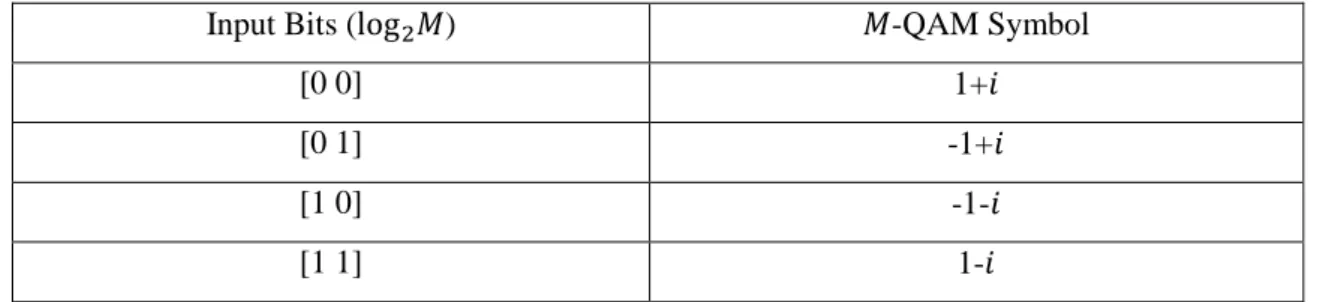
Table 2-1 Gray-coded constellation points for 4-QAM modulation order.
Input Bits (log2𝑀) 𝑀-QAM Symbol
[0 0] 1+𝑖
[0 1] -1+𝑖
[1 0] -1-𝑖
[1 1] 1-𝑖
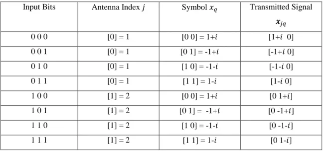
Table 2-2 Mapping process for 2 × 4 4-QAM SM system.
Input Bits Antenna Index 𝑗 Symbol 𝑥𝑞 Transmitted Signal
𝒙𝑗𝑞
0 0 0 [0] = 1 [0 0] = 1+𝑖 [1+𝑖 0]
0 0 1 [0] = 1 [0 1] = -1+𝑖 [-1+𝑖 0]
0 1 0 [0] = 1 [1 0] = -1-𝑖 [-1-𝑖 0]
0 1 1 [0] = 1 [1 1] = 1-𝑖 [1-𝑖 0]
1 0 0 [1] = 2 [0 0] = 1+𝑖 [0 1+𝑖]
1 0 1 [1] = 2 [0 1] = -1+𝑖 [0 -1+𝑖]
1 1 0 [1] = 2 [1 0] = -1-𝑖 [0 -1-𝑖]
1 1 1 [1] = 2 [1 1] = 1-𝑖 [0 1-𝑖]
In the Table 2-2, a 2 × 4 4-QAM SM system is considered, with a spectral efficiency of 3 b/s/Hz. The first bit activates the antenna index 𝑗 and the last two bits select the symbol 𝑥𝑞. The mapped bits are transmitted via a single transmit antenna 𝑗, which was activated by the antenna index.
The transmit vector of the scheme is expressed as [7]:
16
𝒙𝑗𝑞= [0 0 … 𝑥𝑞… 0]𝑇 (2-1)
Considering a 2 × 4 4-QAM SM system with 𝑚 = 3 b/s/Hz, first, log2(𝑁𝑇) is used to select the active transmit antenna out of the two available transmit antennas. Likewise, log2(𝑀), is used to modulate the 4-QAM constellation symbol 𝑥𝑞. The transmit vector 𝒙𝑗𝑞 of dimension 𝑁𝑇× 1is transmitted via the selected active transmit antenna 𝑗 over channel 𝑯 of i.i.d entries with dimension 𝑁𝑅× 𝑁𝑇 with 𝐶𝑁 (0,1) distribution, experiencing AWGN 𝒏 of 𝑁𝑅 × 1 dimension, with i.i.d entries of 𝐶𝑁 (0,1) distribution, such that the received signal 𝒚 becomes:
𝒚 = √𝜌𝑯𝒙𝑗𝑞+ 𝒏 (2-2)
where 𝜌 is the average SNR at each receive antenna.
Assuming the 𝑗𝑡ℎ antenna is used for transmission, the received signal can be rewritten as:
𝒚 = √𝜌𝒉𝑗𝒙𝑗𝑞+ 𝒏 (2-3)
where 𝑗 ∈ [1: 𝑁𝑇], 𝑞 ∈ [1: 𝑀] and 𝜌 denotes the average SNR and 𝒉𝑗 is the 𝑗𝑡ℎ column of the channel 𝑯.
An estimate of the transmit antenna index with the estimated modulated symbol are detected optimally using ML at the receiver to demodulate the transmitted signal, assuming the full knowledge of the channel is known at the receiver. Optimal detection for SM will be discussed in the next sub-section.
2.1.1 Optimal Detection for Spatial Modulation
The transmitted signal is detected at the receiver by estimating the transmit antenna index 𝑗 used for transmission and the modulated symbol 𝑥𝑞 by searching the whole signal space 𝑀
𝑗𝑡ℎ Position
1𝑠𝑡 Position 𝑁𝑇𝑡ℎPosition
17
constellation points and 𝑁𝑇 transmit antennas, i.e. (𝑁𝑇𝑀). Since, SM encodes data to its antenna index and the modulated symbol [16].
The estimates are then fed into the SM de-mapper to recover the transmitted bits, using the SM mapping table (Table 2-1 and Table 2-2) in a reverse mapping process. ML approach is employed to jointly detect the transmitted symbol and the antenna index. This is given as [7, 16]:
[𝑘, 𝑥𝑞̂] = argmin (‖𝒚 − √𝜌𝑯𝒙𝑞‖𝐹2) (2-4)
[𝑘, 𝑥𝑞̂] = argmin (√𝜌‖𝒈𝑗𝑞‖𝐹2− 2Re{𝒚𝐻𝒈𝑗𝑞}) (2-5)
where 𝒈𝑗𝑞= 𝒉𝑗𝑥𝑞̂ and is the transmit antenna index and the estimated transmitted symbol, respectively.
2.2 Performance Analysis for Spatial Modulation
The performance analysis for the average BER ML-based SM, was derived in closed-form expression in [16]. The analysis in [16] is only applicable to binary phase shift keying (BPSK) modulation. However, in [7, 8], the theoretical analysis for square M-QAM SM was derived in closed-form expression to quantify the average BER performance of the system.
In this section, a lower bound approach is employed to compute the theoretical analysis for SM similar to [8], considering the symbol estimation error and antenna index estimation error independently.
In [8], the overall probability of error for SM is given as:
𝑃𝑒 = 𝑃𝑎+ 𝑃𝑑− 𝑃𝑎𝑃𝑑 (2-6) [𝑘, 𝑥𝑞̂] = argmin
𝑞∈[1:𝑀] (‖𝒚 − √𝜌𝑯𝑥𝑞‖
𝐹 2)
[𝑘, 𝑥𝑞̂] = argmax
𝑞∈[1:𝑀] (√𝜌‖𝒈𝑗𝑞‖𝐹2− 2𝑅𝑒{𝒚𝐻𝒈𝑗𝑞})
18
where 𝑃𝑎 is the bit error probability of the antenna index considering that the symbol is perfectly detected, while 𝑃𝑑 is the bit error probability of the estimated symbol considering that the antenna index is perfectly detected.
2.2.1 Analysis of Symbol Estimation
In [8, 36], the average symbol error rate (SER) for 𝑀-QAM over a Rayleigh fading channel is given as:
(2-7)
where 𝑎 = 1 − 1
√𝑀, 𝑏 = 3
𝑀−1, 𝜃 =𝑖𝜋
4𝑐 and 𝑐 > 10, and the BER at high SNR is given by:
𝑃𝑑 ≅𝑆𝐸𝑅𝑚 (2-8)
where 𝑚 = log2𝑀.
2.2.2 Analysis of Transmit Antenna Index Estimation
The bit error probability of the transmit antenna index is computed similar to [7, 8]. According to [7], the transmit antenna index is union bounded by:
(2-9)
where P(𝒙𝑗𝑞→ 𝒙𝑗̂𝑞) is the pairwise error probability (PEP) of choosing 𝑥𝑗̂𝑞, given that 𝑥𝑗𝑞 was transmitted. 𝑁(𝑗, 𝑗̂) is the number of bit errors between the transmitted antenna index 𝑗 and the estimated transmit antenna index 𝑗̂.
SER(𝑘) = (𝑎 𝑐[1
2( 2
𝑏𝑝 + 2)𝑁𝑟−𝑎 2( 1
𝑏𝑝 + 1)𝑁𝑟+ (1 − 𝑎) ∑( 2𝑠𝑖𝑛2𝜃
𝑏𝑝 + 2𝑠𝑖𝑛2𝜃)𝑁𝑟+ ∑ ( 2𝑠𝑖𝑛2𝜃 𝑏𝑝 + 2𝑠𝑖𝑛2𝜃)𝑁𝑟
2𝑐−1
𝑖=𝑐 𝑐−1
𝑖=1
])
𝑃𝑎(𝑘) ≤ 1
𝑁𝑡 × 𝑀 × 𝑙𝑜𝑔2(𝑁𝑡)∑ ∑ ∑ 𝑁(𝑗, 𝑗̂) P(𝒙𝑗𝑞→ 𝒙𝑗̂𝑞)
𝑁𝑡 𝑗=1 𝑁𝑡 𝑗̂=1 𝑀 𝑞=1
19
The closed-form of the conditional PEP of the channel matrix 𝑯 is given in [7] as:
P(𝒙𝑗𝑞 → 𝒙𝑗̂𝑞|𝑯) = 𝑃 (‖𝒚 − √𝜌𝒉𝑗̂𝑥𝑞‖𝐹< ‖𝒚 − √𝜌𝒉𝑗𝑥𝑞‖𝐹) = 𝑄(√𝛾) (2-10)
Using 𝑄(𝑥) =1
𝜋∫ exp (− 𝑠2
2sin2𝜃)
𝜋/2
0 𝑑𝜃 and solving for 𝑃𝛾 = ∫ 𝑄(√𝛾)0∞ 𝑑𝛾, the closed-form of (2-10) can be verified to be the same as (18) in [7]. This is formulated using integration by part with moment generating function (MGF) and the alternative form of Q-function, to get the average PEP over a joint distribution of the channel gain and this can be varied to be:
(2-11)
where 𝜇 = 1
2(1 − √𝛼+1𝛼 ) and 𝛼 =𝜌
2|𝑥𝑞|2.
2.3 Numerical Analysis of the Computed Analytical and Simulated BER for Spatial Modulation
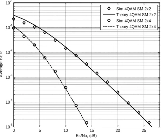
The analytical result for the conventional SM system employing a lower bound approach is computed in this section to validate the Monte Carlo simulation results. The result presented in Figure 2-2 is equipped with two transmit antennas coupled with four and two receive antennas, respectively, employing 4-QAM. The analytical result validates the Monte Carlo simulation results, as they closely match from low SNR to high SNR region. It was observed that, as the number of the receive antenna increases the BER performance of the system improves as expected. At a BER of 10−5 the 2 × 4 4-QAM SM system achieves a gain of approximately 11 dB over 2 × 2 4-QAM SM system.
P(𝒙𝑗𝑞→ 𝒙𝑗̂𝑞) = 𝜇𝑁𝑟 ∑ (𝑁𝑟 − 1 + 𝑘
𝑘 ) [1 − 𝜇]𝑘
𝑁𝑟−1 𝑘=0
20
Figure 2-2 Validation of 4-QAM 2 × 4 and 2 × 2 SM theoretical analysis with the Monte Carlo simulation result
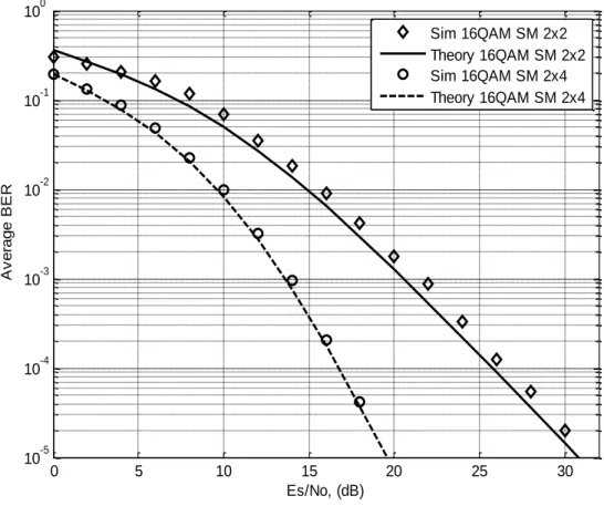
The result presented in Figure 2-3, is equipped with two transmit antennas coupled with four and two receive antennas, respectively, employing 16-QAM. The theoretical result validates the Monte Carlo simulation results. At a BER of 10−5 the 2 × 4 16-QAM SM system achieves a gain of approximately 10 dB over 2 × 2 16-QAM SM system.
0 5 10 15 20 25
10-5 10-4 10-3 10-2 10-1 100
Es/No, (dB)
Average BER
Sim 4QAM SM 2x2 Theory 4QAM SM 2x2 Sim 4QAM SM 2x4 Theory 4QAM SM 2x4
21
Figure 2-3 Validation of 16-QAM 2 × 4 and 2 × 2 SM theoretical analysis with the Monte Carlo simulation result
0 5 10 15 20 25 30
10-5 10-4 10-3 10-2 10-1 100
Es/No, (dB)
Average BER
Sim 16QAM SM 2x2 Theory 16QAM SM 2x2 Sim 16QAM SM 2x4 Theory 16QAM SM 2x4
22
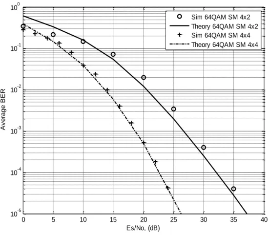
Figure 2-4 Validation of 64-QAM 4 × 4 and 4 × 2 SM theoretical analysis with the Monte Carlo simulation result
In Figure 2-4, at a BER of 10−5 the 4 × 4 64-QAM SM system achieves a gain of approximately 10 dB over 4 × 2 64-QAM SM system, with the theoretical result validating the Monte Carlo simulation results from low SNR to high SNR region.
2.4 Chapter Summary
The system model of a conventional SM system with an optimal detector was presented in this chapter. Similarly, the average BER for 𝑀-QAM SM system with optimal detector over an i.i.d Rayleigh fading channels 𝑯 quantify with the formulated theoretical analysis validating the Monte Carlo simulation results. The analytical framework is shown to be relatively tight with the simulated BER of the SM system as shown in Figure 2-2, 2-3 and 2-4, respectively.
0 5 10 15 20 25 30 35 40
10-5 10-4 10-3 10-2 10-1 100
Es/No, (dB)
Average BER
8 b/s/Hz
Sim 64QAM SM 4x2 Theory 64QAM SM 4x2 Sim 64QAM SM 4x4 Theory 64QAM SM 4x4
23
CHAPTER 3
Quadrature Spatial Modulation 3 Introduction
The criticism of SM, of its data rate enhancement increasing only in logarithm base-two of the total number of transmit antennas compared to other spatial multiplexing techniques, brought about an enhanced spectral efficiency of SM called QSM.
High data rates are highly desirable in wireless communication, but an increase in data rates requires additional transmit antennas, which is expensive. In addition, an increase in the number of required transmit antennas will result to high CC. MIMO systems can achieve high spectral efficiencies with good system reliability [1, 8], this has drawn attention to the system over the years resulting in the use of multiple transmit antennas in an innovative manner to achieve high spectral efficiencies.
In SM [15], a high spectral efficiency is achieved by employing spatial dimension to convey information. Although, SM has a criticism of its data rate being proportional to the logarithm base-two of the number of transmit antennas, when compared to V-BLAST, whose data rate increases linearly with 𝑁𝑇. In improving this criticism, an enhanced spectral efficiency SM called QSM was proposed by Mesleh et al. [33].
QSM, adds an additional dimension to its modulation spatial dimension, i.e. the spatial dimension is extended to the in-phase and quadrature-phase dimensions to enhances the overall spectral efficiency of the system [34]. The constellation symbols are further decomposed into real and imaginary components, while the first dimension transmits the real part of the constellation symbol and the imaginary part is transmitted via the second dimension.
Furthermore, IAS and ICI are completely avoided considering that the in-phase and quadrature- phase components of the constellation symbols are modulated into the cosine and sine carriers, respectively [33, 34].
24 The features of QSM are summarized as follows:
1. QSM improves the criticism of SM with enhanced spectral efficiency with respect to number of transmit antennas [33].
2. In QSM, a single RF chain is employed. Likewise, ICI and IAS are avoided considering the in-phase and quadrature-phase components of the symbol are modulated into the cosine and sine carriers, respectively [33].
3.1 System Model of Quadrature Spatial Modulation
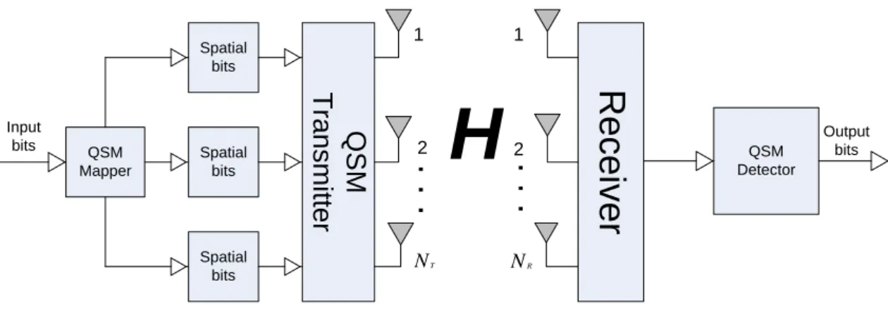
Figure 3-1, depicts a detailed QSM system model equipped with 𝑁𝑇 transmit antennas and 𝑁𝑅 receive antennas.
Figure 3-1 System model for quadrature spatial modulation [37]
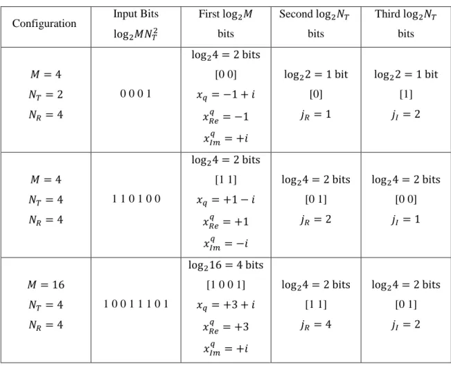
In the QSM system [33] and [34], the spectral efficiency 𝑚 = log2(𝑀𝑁𝑇2), where 𝑀 is the modulation order and 𝑁𝑇 is the total number of transmit antennas. The 𝑀-QAM constellation symbol 𝑥𝑞, 𝑞 ∈ [1: 𝑀] is modulated by log2𝑀 bits and log2𝑁𝑇 bits are used to select the active transmit antenna to transmit the real part of the constellation symbol, while an additional log2𝑁𝑇 bits are used to select the second transmit antenna to transmit the imaginary part of the constellation symbol. Hence, 2log2𝑁𝑇 bits are required to select the active antenna indices needed to transmit the constellation symbol per transmission instant.
The modulated symbol 𝑥𝑞 = 𝑥𝑅𝑒𝑞 + 𝑖𝑥𝐼𝑚𝑞 is further decomposed into real and imaginary components, while the real part of the modulated symbol 𝑥𝑅𝑒𝑞 is transmitted via one of the selected active transmit antenna index 𝑗𝑅 and the imaginary part of the modulated symbol 𝑥𝐼𝑚𝑞 is transmitted via the second transmit antenna index 𝑗𝐼.
QSM Mapper
Spatial bits
Spatial bits Spatial
bits
Q S M T ra n s m itt e r R e c e iv e r
H
1
2
1
2
Input
bits Output
. . . . . .
bitsNT
QSM Detector
NR
25
An example of the mapping process for QSM system is tabulated in Table 3-1:
Table 3-1 Mapping process of QSM system.
Input Bits log2𝑀𝑁𝑇2
First log2𝑀 bits
Second log2𝑁𝑇 bits
Third log2𝑁𝑇 bits 𝑀 = 4
𝑁𝑇 = 2 𝑁𝑅 = 4
0 0 0 1
log24 = 2 bits [0 0]
𝑥𝑞 = −1 + 𝑖 𝑥𝑅𝑒𝑞 = −1
𝑥𝐼𝑚𝑞 = +𝑖
log22 = 1 bit [0]
𝑗𝑅 = 1
log22 = 1 bit [1]
𝑗𝐼= 2
𝑀 = 4 𝑁𝑇 = 4 𝑁𝑅 = 4
1 1 0 1 0 0
log24 = 2 bits [1 1]
𝑥𝑞 = +1 − 𝑖 𝑥𝑅𝑒𝑞 = +1
𝑥𝐼𝑚𝑞 = −𝑖
log24 = 2 bits [0 1]
𝑗𝑅 = 2
log24 = 2 bits [0 0]
𝑗𝐼= 1
𝑀 = 16 𝑁𝑇 = 4 𝑁𝑅 = 4
1 0 0 1 1 1 0 1
log216 = 4 bits [1 0 0 1]
𝑥𝑞 = +3 + 𝑖 𝑥𝑅𝑒𝑞 = +3
𝑥𝐼𝑚𝑞 = +𝑖
log24 = 2 bits [1 1]
𝑗𝑅 = 4
log24 = 2 bits [0 1]
𝑗𝐼= 2
In the Table 3-1,
![Figure 1-1 System Model for a MIMO system [7]](https://thumb-ap.123doks.com/thumbv2/pubpdfnet/10721840.0/18.892.141.782.675.1046/figure-1-1-system-model-for-mimo-system.webp)
![Figure 1-2 System model for low-complexity Euclidean distance transmit antenna selection [19]](https://thumb-ap.123doks.com/thumbv2/pubpdfnet/10721840.0/23.892.277.658.139.469/figure-model-complexity-euclidean-distance-transmit-antenna-selection.webp)
![Figure 2-1 System model for Spatial Modulation [7].](https://thumb-ap.123doks.com/thumbv2/pubpdfnet/10721840.0/30.892.151.785.829.1098/figure-2-1-model-spatial-modulation-7.webp)