Department of Plant Pathology, University of California, Davis, CA, USA
Spatial Analysis Based on Variance of Moving Window Averages
B. M.
B. M. WuWu11,,K. V. SubbaraoK. V.Subbarao11,,F. J. FerrandinoF. J.Ferrandino22andandJ. J. HaoJ. J.Hao33
Author’s addressess:1Department of Plant Pathology, University of California, Davis, c/o US Agricultural Research Station, 1636 East Alisal Street, Salinas 93905, CA;2Plant Pathology and Ecology Department, The Connecticut Agricultural Experiment Station, New Haven, CT 06504;3Department of Plant Pathology, University of California, Davis, CA 95616, USA (correspondence to K. V. Subbarao. E-mail: [email protected])
Received September 19, 2005; accepted February 1, 2006
Keywords:aggregation index, spatial dependency
Abstract
A new method for analysing spatial patterns was designed based on the variance of moving window averages (VMWA), which can be directly calculated in geographical information systems or a spreadsheet program (e.g. MS Excel). Different types of artificial data were generated to test the method. Regardless of data types, the VMWA method correctly determined the mean cluster sizes. This method was also employed to assess spatial patterns in historical plant disease sur-vey data encompassing both airborne and soilborne diseases. The results obtained using the VMWA method were generally different from those obtained with Lloyd’s index of patchiness and beta-binomial distribution methods, were in partial agreement with the results from spatial analysis by distance indices, and were highly consistent with the results from semi-variogram and spatial autocorrelation analysis meth-ods. Results demonstrated that the VMWA method can be applied to many types of data, including bino-mial diseased or healthy plant counts, incidence, sever-ity, and number of diseased plants or pathogen propagules although directional and edge effects may limit its application.
Introduction
Spatial patterns are considered as a manifestation of biological processes, reflecting the interactions among different determining factors. Spatial patterns provide information regarding the mechanisms that bring about these patterns, which can then be applied to improve sampling techniques, and to develop strategies for the management of our environments. Methods to detect and assess spatial pattern and to quantify spa-tial distribution and association among different ele-ments in an ecological system, have received increasing attention in ecological research since the beginning of modern ecology. This in turn has laid a strong founda-tion for a better understanding of the biological
pro-cesses that generate the patterns. Methods for analysing spatial patterns have been developed in a wide variety of disciplines, such as plant communities, statistics, forestry and geostatistics, over the past dec-ades (Clark, 1979; Campbell and Noe, 1985; Madden and Hughes, 1995; Real and McElhany, 1996; Liu, 2001).
A commonly used approach to determine spatial patterns is to compare the observed frequency distribu-tion with theoretical frequency distribudistribu-tions such as Poisson, binomial, negative binomial, Neyman type A, and beta-binomial distributions (BBD) (Hughes and Madden, 1993; Madden and Hughes, 1994). Based on the best fit of observed frequencies to these distribu-tions, a spatial pattern is considered aggregated, ran-dom or uniform (Campbell and Noe, 1985; Campbell and Madden, 1990; Madden and Hughes, 1995). It is generally accepted that for count data, a good fit to the Poisson distribution suggests random distribution (Fisher, 1925), while a good fit to the negative-bino-mial distribution implies heterogeneity (Madden and Hughes, 1995). Similarly, for a binary variable a good fit to the binomial distribution indicates homogeneity while a good fit to the BBD suggests heterogeneity (Madden and Hughes, 1995). The frequency distribu-tion approach has also been extended to calculate indi-ces of aggregation or dispersion. The indiindi-ces that have been commonly used include, Fisher’s variance-to-mean ratio (Fisher, 1925), David and Moore’s index of clumping (David and Moore, 1954), the slope of the log(variance) to log(mean) line in the Taylor’s empir-ical power law (Taylor, 1961), Morisita’s index, Id (Morisita, 1962), Lloyd’s mean crowding and indices of patchiness (LIP) (Lloyd, 1967), the parameter k of the negative-binomial distribution (Elliott, 1977), and the parameter h of BBD (Irwin, 1954; Griffiths, 1973;
Hughes and Madden, 1993; Madden and Hughes, 1994, 1995). Because the methods based on frequency distributions ignore the information about the
loca-www.blackwell-synergy.com J. Phytopathology154, 349–360 (2006)
2006 The Authors
tions of sample sites and their spatial relationship, they reflect only the relationship among individuals within sample units. If the presence of one individual enhan-ces the presence of other individuals within the same sample unit, then the frequency distribution would be determined as aggregated; otherwise, it follows a uni-form or random distribution. The aggregation deter-mined using frequency distribution based methods has often been referred to as heterogeneity (Madden and Hughes, 1995).
Other methods that take into consideration the loca-tion of sample sites have also been developed for char-acterization of spatial patterns. These methods include: spatial analysis by distance indices (SADIE), methods based on quadrat variance, spatial autocorrelation, dis-tance based joint-counts/network method and geosta-tistics.
SADIE (Perry and Hewitt, 1991; Alston, 1994; Perry, 1995) determines an index of aggregation by comparing the observed spatial arrangement with other arrangements derived from it, such as those where individuals are arranged as crowded as possible, those as random as possible, and those as regular as possible. Aggregation detected by SADIE method may be non-random in two different ways, non-random fre-quency distribution of counts regardless of the loca-tions of sample units, and the non-random spatial arrangement of the sample units. Perry and Hewitt (1991) defined Ômove to crowdingÕ as the minimal total number of moves required to move all individuals, one by one and step by step, so that all the individuals fin-ish in the same sample unit. ÔMove to randomnessÕ was also defined similarly, and a test based on the ratio ofÔmove to crowdingÕ and Ômove to randomnessÕ
was proposed as an index for detecting aggregation in spatial patterns. Lately,Ôdistance to regularityÕ (D) was suggested as a replacement to Ômove to randomnessÕ
(Alston, 1994). The approach was further extended to map two-dimensional data, and a new method was developed to estimate the initial focus of a cluster based on the movements (Perry, 1995).
Blocked quadrat variances (BQV) (Greig-Smith, 1952) method determines cluster size by identifying the peak of mean Ôlocal varianceÕ (mean squared difference between adjacent blocks) as quadrat sizes increase by combining two contiguous quadrats to form a new quadrat. The two major drawbacks with the BQV method are that the block sizes must be some power of 2, and that the starting position of blocking can affect the results. The two-term local quadrat variance method (Hill, 1973) offers more flexibility to the block size, and reduces the effects of the starting position. However, quadrats are still blocked along the belt transect and edge effects are important. Therefore, the variance is affected not only by distance (spacing) but also by the block size. This disadvantage was over-come in the paired-quadrat variance and random paired-quadrat variance methods, in which the vari-ance was calculated for all possible paired quadrats along the belt at a given spacing for the former or for
randomly selected paired quadrats for the latter (Goodall, 1974). The quadrat variance methods pro-vide informative results of aggregation and the size of clumps and are independent of the assumption of dis-tributions. However, the calculations become compli-cated for two-dimensional data sets.
Spatial autocorrelation, distance-based joint-counts methods and geostatistics are all similar. Spatial auto-correlation can be defined as a spatial property that the presence of some quality at one sample site (quad-rat or location) makes its presence at proximal sample sites more or less likely (Cliff and Ord, 1973). Proxim-ity can be determined by the connection between the two samples sites, such as distance, lag distance, vector or other criterion. Unlike methods based on negative binomial and Poisson distributions, which can only be used for discrete count data, the spatial autocorrela-tion analysis can be conducted on any type of data, continuous or discrete. Data used in spatial autocorre-lation can be point based, area based or even without information on the exact shape of areas. The two most common coefficients in spatial autocorrelation analysis are Moran’s I, which is based on sum over the cross-product of deviations from mean, and Geary’s c, which is based on sum of the squared difference (Moran, 1950; Geary, 1954). Joint-counts method, which has also been referred as distance-based meth-ods and neighbour networks, is an analysis for discrete data based on point pairs (Campbell and Madden, 1990; Real and McElhany, 1996; Liu, 2001). There are a number of ways for point pairing, such as Gabriel connectedness (Gabriel and Sokal, 1969), the nearest neighbour (Clark and Evans, 1954; Pielou, 1959), and one- or two-dimensional distance class (Gray et al., 1986; Nelson et al., 1992; Ferrandino, 1996). After establishing connectedness, the number (or average distance) of each type of joint is counted and this observed value is then compared with the expected one under the assumption of randomness. Geostatistical techniques, originally developed for use in mining (Clark, 1979), can be used for both continuous and discrete variables, and require less stringent assump-tions of stationarity compared with spatial autocorre-lation techniques. In geostatistics, spatial dependence can be analysed directionally or omnidirectionally, and represented as semivariogram or correlogram. Semi-variogram calculates semivariance against each lag dis-tance (a vector h), in which semivariance is defined as half of mean squared difference between all point pairs (p, p+h) separated by h. In a correlogram, the linear (Pearson’s) correlation coefficients between point pairs separated by a vector h are plotted against vectorh or lag distance at different directions.
ever to implement. However, few spatial techniques have been developed based on GIS data. An instinct-ive method of determining whether a spatial data set is aggregated by human beings is to visually scan through the spatial data and determine whether the data are aggregated based on whether the densities of individuals or mean value varies ÔsignificantlyÕ among different subareas. In GIS software, such as GRID module of Arc/Info [Arc/Info version 7; Environmen-tal Systems Research Institute (ESRI), Redlands, CA, USA] and ArcGIS (ArcGIS version 9; ESRI), a com-mon function called smoothing filter or focal mean, in which the value at the centre of the moving window is computed as a simple arithmetic average of the other values in the window, is very similar to the scanning movement of human eyes and with a mental calcula-tion of densities or mean values. A spatial analysis method based on moving window averaging will elim-inate the importance of the arbitrary and happenstan-tial positioning of contiguous quadrats, which inflate the error for all fixed quadrat methods. Such a method will be easy to interface with GIS programs, and establish a foundation for developing other spatial analysis techniques in the future.
Therefore, our aim was to develop a method that is based on moving window averaging. Variance of the resulted averages is used to determine if the average varies significantly at different locations. The relation-ship between the change of variance as the moving window changes size and the average cluster size of spatial data are analysed. The method, although not described in detail, has been used previously (Bhat et al., 2003) in analysis of spatial patterns, and briefly discussed in a review (Wu and Subbarao, 2005).
Materials and Methods
Spatial dependence and variance of moving window averages Generally, forn variables (Xi,i¼1,…,n) each with a variancev, the variance of their mean
Y ¼X n
i¼1
Xi
n
can be calculated as:
varðYÞ ¼
Pn
i¼1varðXiÞ þ P
i6¼jcovðXi;XjÞ
n2 ; ð1Þ
where var(X)¼v, and cov(Xi,Xj) denotes covariance between Xi and Xj (i „ j). This suggests that the
variance of averages ofnsamples isv/nif the samples are all randomly distributed and have a variance v (cov(Xi,Xj¼0 for i „ j), the variance of averages is
greater than v/n if they are aggregately distributed or positively correlated with each other (cov(Xi,Xj) > 0 for i „ j), and smaller than v/n if they are uniformly
distributed (cov(Xi,Xj) < 0). Averaging by moving an n·n window is similar to calculating averages of n2
variables with the same variance and mean, the devi-ation of variance of the averages from v/n2, can therefore be used as a measure of spatial dependency
within the window. To use an index (or a set of indices) as a measure of the spatial dependency over the whole data set, first, a ÔstationaryÕ assumption is needed, i.e. there exists a general or universal degree of dependency over the whole data set. The spatial dependency among the points within a moving window either does not change as the position of the moving window changes through the data set or they are additive and their mean represents the degree of spatial dependency over the whole data set. This is the basis of using a single index (or a set of indices) for the whole data set. Secondly, because a large window contains smaller windows, the spatial dependency at smaller windows will be carried over to larger windows. To quantify the carryover effects, an ÔisotopicÕ assumption is needed: the spatial dependency between any point pair in a large window is the same as in the smaller windows as long as the minimum size of window to cover the two points remains the same, regardless of the direction of the vector linking the two points, and the overall spatial dependency within a window can therefore be decom-posed as the sum of the spatial dependency between all the possible point pairs. Based on these two assump-tions, the new method of spatial analysis was developed using the variance of moving window averages (VMWA), the detailed mathematical derivations are given in the Appendix.
Calculation of spatial dependency indices
The calculation of dependency indices of VMWA can be carried out easily in GIS or in Microsoft Excel fol-lowing a simple procedure.
Step 1: arrange the original two-dimensional data set, one sample point per cell;
Step 2: move a window (size 1·1, 2· 2, 3·3,
etc.) cell by cell two-dimensionally and calculate the average of samples within the moving win-dow to generate a new data set by assigning the average to the center cell (or left upper cell clo-sest to the centre) of the moving window;
Step 3: calculate mean and variance of original data and the new data sets derived from different sizes of moving windows;
Step 4: assess the edge effects based on the change of overall mean, dramatic changes in mean suggest strong edge effects or the values at edges are very different from the values at other places;
Step 5: calculate spatial dependency index at each window size based on variance of the aver-ages at different window sizes by solving equa-tions (equaequa-tions 6 & 7 in the Appendix);
Step 6: interpret the results: if the index > 0, then aggregated; if the index¼0, then random; otherwise (index < 0) uniform distribution.
Application of the VMWA method to artificial 0–1 data The VMWA method was first tested with artificially generated binary data with regular, random and 351
aggregated distributions. Six regularly distributed bin-ary data sets were generated for a 20·20 field.
Among them, examples 1 and 2 consisted of alternat-ively arranged lines of 0 and 1 s, diagonally and hori-zontally respectively. In examples 3–6, the 1 s was only located at the four corners of 3·3 to 6·6 windows,
and the remainder of the cells were all 0 s, so that no two 1 s were located in any 2·2 (to 5·5) window.
Random 0–1 data sets were generated based on an assumption that each sample site has a value of 0 or 1 randomly with P(x ¼1) ¼0.1–0.9 (500 data sets were generated at each P-value), and that different sample sites are independent of each other. Aggregated 0–1 data were generated using commonly used Neyman– Scott cluster process (Cressie, 1991), with the first step being the random generation of 1, 2, 4, 10 disease foci (infected plants have a value¼1) in a field with 20·20 plants. Then, whether a plant becomes infected
from each of the foci was determined (simulating 200 times of infection) according to the distance (r) from the disease focus: if the distance was farther than the influence range (denoted here the maximum distance that pathogen propagules could be disseminated) parameter R or the plant has already been infected, then no action was taken, otherwise the plant had the potential of getting infected at a probability of P¼e)r/R/2prR (van den Bosch et al., 1988). For each focus number, 400 data sets were generated for each influence range fromR¼1 toR¼7.
Application of the VMWA method to artificial count data Artificial count data with different distributions were generated and used to test the VMWA method. Ran-dom distribution data sets were generated assuming that each sample unit consisted of 20 individuals and each of them randomly (independently) became dis-eased at a probability P¼0.1–0.9 or otherwise remained healthy (500 data sets were generated at each P-value). Aggregated data sets were generated using a Neyman–Scott cluster process similar to the above. First, 10 disease foci (sample units) were randomly generated in a 20·20 field. Then, disease (unlimited)
was reproduced at each sample unit around each of these foci according to a given disease gradient func-tion based on its distance r from the centre of these foci, D(r)¼e)r/R/(2prR). At each focus number, 400 data sets were generated for each influence range from R¼1 to R¼16. Similar simulation was also carried out in a 40·40 field with influence range from R¼1
toR¼36.
Application of VMWA to historical survey data
The VMWA method was also employed to assess the spatial patterns in historical data from disease surveys and compared with the results obtained from other methods.
First, the number of lettuce plants infected by Bremia lactucaefrom historical disease surveys in three fields, in which each sample unit consisted of 10 plants, and sample sites were 20 m apart within a row
and across rows (Wu et al., 2001), was analysed using VMWA, BBD (Madden and Hughes, 1994), SADIE (Perry, 1995, 1998) and spatial autocorrelation soft-warelcor2 (Gottwald et al., 1992).
Secondly, the number of microsclerotia of Verticil-lium dahliae per gram soil from cauliflower fields, the number of plants infected by V. dahliae and the dis-ease severity in the same field sites from a previous study (Xiao et al., 1997) were analysed using the VMWA method. Each site was divided into 8·8
con-tiguous quadrats, 2·2 m each (2-m length on two
rows of cauliflower plants). The results obtained with the VMWA method were compared with those obtained with LIP, BBD, semivariogram and SADIE methods, as applicable to each data set.
The VMWA method was also used to analyse his-torical data from disease surveys on pepper wilt caused by V. dahliae (Bhat et al., 2003). The original data of healthy or diseased status for every individual plant, was used in this analysis instead of the 20-plant quad-rats reported in the study (Bhat et al., 2003). No com-parison of the results with LIP, BBD, lcor2, SADIE or semivariogram methods was made because none was applicable to these large binary data sets with missing data at some sample sites.
Results
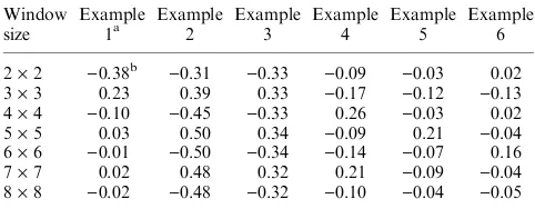
Application of the VMWA method to artificial 0–1 data For the six examples of regularly distributed 0–1 data, the index calculated using the VMWA method cor-rectly reflected the spatial pattern. In examples 1 and 2, the spatial dependency index was negative at mov-ing window size 2·2, and positive at 3·3, consistent
with the one-line wide gap between any two lines of 1 s (Table 1). In examples 3–6, the indexes remained negative or almost zero when moving windows were smaller than the minimum window sizes (3·3 to
6·6 in examples 3–6) required to cover any two 1 s,
Table 1
Spatial dependency indices at different window sizes calculated using a method based on variance of moving window averages for artificial binary data with a regular distribution
Window size
Example
1a Example2 Example3 Example4 Example5 Example6
2·2 )0.38b )0.31 )0.33 )0.09 )0.03 0.02
3·3 0.23 0.39 0.33
)0.17 )0.12 )0.13
4·4 )0.10 )0.45 )0.33 0.26 )0.03 0.02
5·5 0.03 0.50 0.34
)0.09 0.21 )0.04
6·6 )0.01 )0.50 )0.34 )0.14 )0.07 0.16
7·7 0.02 0.48 0.32 0.21
)0.09 )0.04
8·8 )0.02 )0.48 )0.32 )0.10 )0.04 )0.05
aAll example data sets were composed of 20·20 data points each
with a value 0 or 1. In examples 1 and 2, 0 and 1 s were arranged in alternative lines, diagonal and horizontal respectively. In examples 3–6, 1 s were only located at the four corners of 3·3 to 6·6 win-dows in the order, and the rest were all 0 s, so that no two 1 s were located in any 2·2 to 5·5 (in the same order) windows.
b
and became positive when the moving windows were at the minimum sizes (Table 1).
Regardless of the incidence, the VMWA method correctly classified the spatial patterns for randomly distributed 0–1 data sets as the value of the index was close to zero and varied little in the 500 simulations at each incidence (Table 2).
As for aggregated 0–1 data, the VMWA method correctly reflected the ranges used in epidemic simula-tions when the ranges were shorter than 5 in a 20·20
field regardless of whether the number of disease foci was 1, 2, 4 or 10 (Fig. 1a–d). The indices were positive for moving window 2· 2, remained positive till the
window size was equal to influence range +1, and decreased to zero at the window size equal to range +2 (Fig. 1a–d). However, as the range increased beyond 5, the index curve became slightly flatter. For the small moving windows, the index topped off at range 3–4, and began to decrease as the range increased further (Fig. 1a–d) perhaps because the cen-tre of the disease foci becomes a plateau as the range increased.
Application of the VMWA method to artificial count data Simulations of count data (number of diseased plants) showed that the VMWA method correctly identified the spatial pattern as disease incidence ranged from 10% to 90%. The indices were close to zero and var-ied little (Table 3). As for the simulated aggregated data, the VMWA method correctly reflected the ranges used in simulation of the epidemics when the ranges were small. The index curves changed less after the range increased beyond 10 in a 20·20 field (Fig. 2a)
and 20 in a 40·40 field (Fig. 2b). These curves were
slightly different from the curves for 0–1 data in Fig. 1a–d in that for count data, there was no decrease in the value of the index at small moving windows as the range increased. This difference was perhaps because the centre of a disease focus never became a plateau (unlimited disease level) as the range increased in simulation, unlike the simulation of 0–1 data.
Application of VMWA to historical survey data
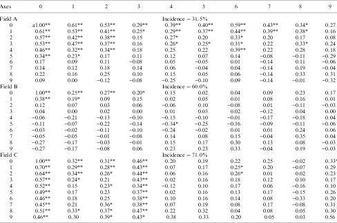
For the number of lettuce plants infected by B. lactu-cae, the VMWA method detected positive (positive index) association among the sample sites within a win-dow size of 4–5 in all three fields (Table 4). Therefore, it determined that the distributions were aggregated. The field with 60% incidence had the lowest degree of aggregation, and the smallest cluster size among the three fields. These results were highly consistent with the results from the previous semivariogram analysis (Wu et al., 2001) and results from lcor2 (Table 5). Results from SADIE (Perry, 1995, 1998) and BBD ana-lysis (Madden and Hughes, 1994) also defined that dis-eased plants in the three fields were all aggregated (Table 4), suggesting a positive association not only within sample units but also across sample units.
For the number of microsclerotia of V. dahliae per
gram soil from cauliflower fields, weak aggregation Ta
ble
(with positive, but small indexes) was detected by the VMWA method in sites A1, A2, B1, B2, B3, C2 and C3, but not in the other sites (Table 6), which suggests weak association between the numbers of microsclero-tia across sample sites. The results were highly consis-tent with the previous results from semivariogram analysis (Xiao et al., 1997), but different from the results of LIP tests, which showed a LIP value >1 in all the sites, indicating an aggregated distribution of microsclerotia within sample units (Xiao et al., 1997). The results also differed from those obtained with SA-DIE, which showed aggregated spatial patterns of microsclerotia only in sites A2 and C2 (Table 6). As for the number of cauliflower plants infected by V. dahliae (Xiao et al., 1997), the VMWA method detec-ted aggregadetec-ted distributions not only in field sites A1, A2 and B3 in which BBD detected aggregation previ-ously (Xiao et al., 1997), but also in sites B1, B2, C1, D1 and D3 (Table 6) in which aggregation was not detected previously by BBD (Xiao et al., 1997). The results were partly consistent with the results obtained from SADIE method, which also defined aggregated distribution for diseased plants in sites B1, C1 and D1, but not in sites B2, B3 and D3. Furthermore, no aggregation was found by the VMWA method (Table 6) in field sites A3 and C3 where aggregation
was defined previously by BBD method (Xiao et al., 1997), but not by SADIE method (Table 6). When dis-ease severity was analysed, aggregation was detected in four of the six field sites examined (Table 6). The LIP, BBD and SADIE methods were not suitable for these data sets.
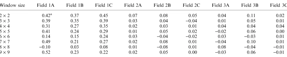
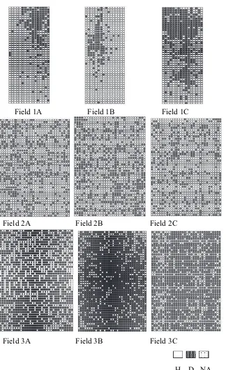
As for the binary data of healthy or diseased (infec-ted by V. dahliae) pepper plants, the VMWA method revealed strong aggregation in field sites 1A, 1B and 1C, weak aggregation in field sites 2A, 2B and 3B (Table 7), and random distribution in the other three sites 2C, 3A and 3C, highly consistent with the visual impression of the maps (Fig. 3).
Discussion
Based on the above analyses, the VMWA method pos-sesses certain advantages over currently available tech-niques for spatial pattern analysis. First, choice of proper software for spatial pattern analysis has long been the bane for average users in spatial pattern analy-sis because of the variety of programs available, the level of computer knowledge required to use these programs and their applicability being restricted to certain types of data. This has resulted in many cases of inappropriate application of spatial analysis methods. The VMWA method can be applied to many types of data including –0.2
0 2 4 6 8 10 0 2 4 6 8 10
0 2 4 6 8 10 0 2 4 6 8 10
0.0 0.2 0.4 0.6 0.8
Window size
R1 R2 R3 R4 R5 R6 R7
–0.2 0.0 0.2 0.4 0.6 0.8
Window size
R1 R2 R3 R4 R5 R6 R7
–0.2 0.0 0.2 0.4 0.6 0.8
Window size
R1 R2 R3 R4 R5 R6 R7
–0.2 0.0 0.2 0.4 0.6 0.8
Window size
R1 R2 R3 R4 R5 R6 R7
(a) (b)
(c) (d)
In
In
In
In
Fig. 1 Spatial analysis of the aggregated binary data using the variance of moving window averages method. Data were artificially generated using a Neyman–Scott cluster process with 1 (a), 2 (b), 4 (c) and 10 (d) disease foci. Each index (In) in the figure was the average in four
bina
Averages and SDs of spatial dependency indices at different window sizes calculated using a method based on the variance of moving window averages for simulated number of diseased plants with random distribution and different incidence levels
Incidence (%)
Spatial dependency indices at different window sizes
2·2 3·3 4·4 5·5 6·6 7·7 8·8 9·9 10·10
The average of spatial dependency indices in 500 simulations. Positive values indicate positive association negative values indicate negative association, and zero values indicate random distribution
or independence. Each data set, consisted of 20·20 sample units, was generated assuming that each sample unit consisted of 20 individuals and each of them randomly (independently) became
dis-eased (with P¼0.1–0.9) or remained healthy.
sets (when edge effect is ignorable) used in this study. The VMWA method theoretically differs from spatial autocorrelation in that only the average association over all directions is given in the outputs of VMWA while the latter can also give the association for each direction, and that the VMWA method uses a window size that is slightly different from the distance (vector) used in autocorrelation (or semivariogram). Because of these, compared with spatial autocorrelation and
semi-variogram methods, the VMWA method is more suit-able when data sets are small, and when the topological relationship between any two sample sites is more important than the physical distance and ori-entation between them. It should also be noted that the number of calculations for moving average is con-siderably fewer than the number of calculations for distance between any two pairing points, as the size of a data set increase. This is also a significant benefit of the VMWA method as more and more raster data are becoming available, and the resolution of the data increasing over years. For example, for a data set com-posed of 1.0·108 (10 000·10 000) points, spatial
autocorrelation needs to calculate distance for approxi-mately 5.0·1015 point pairs while the VMWA
method, at maximum, needs to calculate 1.0·1012
averages. Furthermore, if we are only interested in the spatial dependence at a smaller scale, such as within a 500·500 or smaller window, the number of averaging
calculations can be further reduced to 5.0·1010. This
would significantly reduce the computing time, and make it feasible to do spatial analysis for data sets covering large areas and with high resolutions.
The VMWA method is, to some extent, also similar to the quadrat variance methods. The latter calculate the Ôlocal varianceÕ between adjacent blocks or paired quadrats, and then calculate the overall average Table 4
Characterization of spatial patterns of lettuce plants showing downy mildew symptoms in 1998 surveys (field A–C) using the variance of moving window averages (VMWA), spatial analysis by distance indi-ces (SADIE) and beta-binomial distributions (BBD) methods
Method
Indices/ coefficients
Field A (31.5%)
Field B (60.0%)
Field C (71.0%)
VMWA Ia
2 0.58 0.30 0.49
I3 0.51 0.02 0.18
I4 0.24 0.15 0.40
I5 0.18 )0.07 0.05
SADIE Ia 3.32*
b
1.56* 3.20*
BBD h 0.41* 0.16* 0.36*
D 3.66* 2.26* 3.40*
a
I2–I5 denote spatial dependency indices at window sizes 2·2,
3·3, 4·4 and 5·5 respectively. Positive values indicate positive association, negative values indicate negative association, and zero values indicate random distribution, independence.
bI
a,handDvalues followed by asterisk were significant (P < 0.05).
Table 5
Analysis of spatial patterns of lettuce plant showing downy mildew in 1998 surveys (fields A–C) usinglcor2
Axes 0 1 2 3 4 5 6 7 8 9
Field A Incidence¼31.5%
0 a1.00** 0.61** 0.53** 0.29** 0.39** 0.40** 0.59** 0.43** 0.34* 0.27 1 0.61** 0.53** 0.41** 0.25* 0.29** 0.37** 0.44** 0.39** 0.38* 0.16
2 0.57** 0.42** 0.38** 0.15 0.27* 0.20 0.33* 0.20 0.17 0.08
3 0.53** 0.47** 0.37** 0.16 0.26* 0.25* 0.31* 0.22 0.33* 0.24
4 0.46** 0.32** 0.34** 0.18 0.25 0.22 0.39** 0.22 0.28 0.18
5 0.34** 0.23* 0.17 0.11 0.12 0.07 0.14 )0.08 )0.11 )0.29
6 0.17 0.09 0.11 )0.08 0.05 )0.05 0.01 )0.14 0.11 )0.06
7 0.14 0.12 0.18 0.14 0.06 )0.04 0.04 )0.14 0.19 )0.04
8 0.22 0.16 0.25 0.10 0.15 0.05 0.06 )0.14 0.33 0.31
9 0.09 0.00 )0.12 )0.08 )0.25 )0.10 0.09 )0.14 )0.01 )0.32
Field B Incidence¼60.0%
0 1.00** 0.25** 0.27** 0.20* 0.15 0.02 0.04 0.09 0.23 0.17
1 0.38** 0.19* 0.09 0.15 0.02 0.05 0.01 0.08 0.16 0.01
2 0.12 0.07 0.03 0.06 )0.06 0.10 )0.08 0.01 )0.11 )0.03
3 0.04 0.00 0.02 0.00 0.01 0.03 0.02 )0.12 0.04 0.00
4 )0.06 )0.21 )0.13 )0.10 )0.15 )0.10 )0.01 )0.17 )0.18 0.04
5 )0.11 )0.07 )0.22 )0.14 )0.34* )0.25 )0.16 )0.09 )0.11 )0.06
6 )0.03 )0.02 )0.11 )0.10 )0.24 )0.02 0.01 0.01 0.24 0.06
7 )0.05 )0.05 )0.01 )0.08 0.14 0.08 0.15 )0.04 0.35 0.04
8 )0.27 )0.17 )0.03 )0.01 0.15 0.17 0.30 0.13 0.08 )0.03
9 )0.27 )0.17 )0.08 0.06 0.23 0.23 0.33 )0.04 0.19 )0.03
Field C Incidence¼71.0%
0 1.00** 0.32** 0.31** 0.46** 0.20 0.19 0.22 0.25 )0.02 0.33*
1 0.70** 0.29** 0.28** 0.43** 0.07 0.17 0.25* 0.20 )0.07 0.29
2 0.64** 0.34** 0.26* 0.44** 0.06 0.16 0.26* 0.01 0.02 0.23
3 0.57** 0.24* 0.21 0.43** 0.02 0.16 0.18 0.12 0.10 0.17
4 0.52** 0.15 0.23* 0.34** )0.12 0.10 0.17 0.06 )0.16 0.10
5 0.49** 0.17 0.23 0.37** 0.02 0.16 0.13 0.17 )0.15 0.26
6 0.46** 0.18 0.25 0.38** 0.10 0.16 0.14 0.08 )0.33 0.20
7 0.45** 0.21 0.36* 0.38** 0.07 0.19 0.08 0.17 )0.08 0.31
8 0.51** 0.33* 0.37* 0.47** 0.22 0.32 0.04 0.08 0.05 0.30
9 0.46** 0.30 0.39* 0.43* 0.38 0.33 0.20 0.05 0.03 0.56
(Greig-Smith, 1952; Hill, 1973; Goodall, 1974; Ludwig and Goodall, 1978). For example, at block size 1, the
Ôlocal varianceÕ can be calculated differently in different quadrat variance methods, such as
ðx1x2Þ2þ ðx3x4Þ2þ. . .. . .
2 or
ðx1x2Þ2þ ðx2x3Þ2þ ðx3x4Þ2þ. . .. . .
2
and more. Taking the first formula as an example and assuming that the mean of the data set ism, it can be further rewritten as:
P
ðxmÞ2
2 ½ðx1mÞðx2mÞ þ ðx3mÞðx4mÞ þ. . .:
It becomes clear that the second part of the formula is a portion of total cross-product at distance 1 (one-dimensional data). Because calculation of the Ôlocal varianceÕ becomes complicated as the block size increases, the quadrat variance methods become com-plicated as well. Besides, the results of the methods are usually affected by the starting place of quadrat and
block size, and it is difficult to use these methods in two-dimensional data sets, which are more common in nature. The VMWA method, in contrast, is intrinsically more suitable for two-dimensional data than the traditional quadrat variance methods because the calculation of average is very easy within each moving window. Moreover, moving the windows two-dimen-sionally makes the results of the variance reflecting the whole data set better, and is less affected by local variation or by the starting position of the moving windows. The partition of variance for a big moving window into variance at smaller windows solved the carryover problem satisfactorily. These together make the VMWA method more stable as well as more accurate.
As with most other methods, there are also certain limitations with the VMWA method. As stated above, it cannot detect directional differences. Instead, it gives an average degree of spatial association between two samples. It is inappropriate to use this method when directional effects are significant because the calculation of spatial dependency index relies upon the ÔisotopicÕ assumption. In addition to this limita-tion of direclimita-tional effect, edge effect is another factor Table 7
Spatial dependency indices at different window sizes for spatial patterns of pepper plants infected byVerticillium dahliaein 1998 surveys at fields 1, 2 and 3 calculated using the variance of moving window averages method
Window size Field 1A Field 1B Field 1C Field 2A Field 2B Field 2C Field 3A Field 3B Field 3C
2·2 0.42a 0.37 0.45 0.07 0.08 0.05 0.04 0.11 0.02
3·3 0.39 0.35 0.39 0.03 0.04
)0.04 0.01 0.05 0.01
4·4 0.31 0.27 0.35 0.02 0.03 0.01 0.04 0.04 0.04
5·5 0.41 0.24 0.29 0.01 0.05 0.02
)0.02 0.06 0.00
6·6 0.14 0.15 0.24 0.03 )0.04 )0.02 0.03 )0.03 0.01
7·7 0.49 0.21 0.27 0.02 0.08 0.01 )0.04 0.10 0.01
8·8
)0.10 0.03 0.08 0.01 )0.08 0.01 0.08 )0.04 )0.01
9·9 0.52 0.23 0.22 0.02 0.05 0.00 )0.03 0.06 )0.01
aPositive values indicate positive association, negative values indicate negative association, and zero values indicate random distribution,
inde-pendence. Table 6
Characterization of spatial pat-terns in number of microsclerotia ofVerticillium dahliae, number of cauliflower plants infected by the pathogen and disease severity (Xiao et al., 1997) using the vari-ance of moving window averages (VMWA), Lloyd’s indices of pat-chiness (LIP) or beta-binomial distributions (BBD) (Madden and Hughes, 1994) methods
Plots
Number of microsclerotia Number of diseased plants Disease severity
VMWAa LIP Ic
a VMWA h
b
Ic
a VM
A1 0.10 2.17 1.234 0.17 0.055* 1.682*
A2 0.13 1.15 1.533* 0.44 0.145* 2.481* A3 )0.01 1.08 1.273 0.04 0.047* 0.941
B1 0.07 1.10 1.101 0.15 0.019 1.543*
B2 0.12 1.06 1.265 0.16 0.017 1.147
B3 0.11 1.09 0.929 0.10 0.056* 1.272
C1 )0.01 1.07 0.909 0.13 0.007 1.618* 0.38
C2 0.10 1.17 1.618* )0.06 0.010 0.802 0.13
C3 0.07 1.11 1.120 )0.02 0.040* 1.095 0.12
D1 )0.08 1.09 1.129 0.27 0.004 2.069* 0.13
D2 )0.01 1.06 1.138 )0.18 0.011 0.823 0.04
D3 )0.06 1.04 1.175 0.07 0.018 1.308 )0.13
a
Spatial dependency index at window size of 2 (two nearby sample sites) using VMWA method. Posit-ive values indicate positPosit-ive association, negatPosit-ive values indicate negatPosit-ive association, and zero values indicate random distribution, independence.
bA value from BBD followed by
Ô*Õindicates an aggregation of diseased plants (Xiao et al., 1997).
c
Ia from spatial analysis by distance indices method followed by Ô*Õ indicates an aggregation
(P < 0.05).
357
that may limit the use of VMWA method because a moving window consists of fewer pairs far apart at the edges than at the center, and the number of pairs affected increases as the window size increases. Although another method was developed as a com-parison, it was found that the edge effect, in general, tends to cause the aggregation index to fluctuate. In cases where edge effect was not significant, the two methods ended in very similar results (results not shown).
The VMWA method has also great potential for interfacing with GIS because moving window averaging
is a common function in GIS, such as in ArcGIS, a widely used GIS software. This feature makes VMWA very easy to carry out although more studies are needed to adapt this method into GIS. To further increase its flexibility, it is also possible to use different shapes of moving windows, such as rectangle windows to deter-mine the shape of clusters in addition to the average cluster size (see equations 12–14 in the Appendix).
References
Alston R. Statistical analysis of animal populations. PhD thesis, Kent, University of Kent, 1994.
Field 1A
Field 1B
Field 1C
Field 2A
Field 2B
Field 2C
Field 3A
Field 3B
Field 3C
H
D
NA
Bhat RG, Smith RF, Koike ST, Wu BM, Subbarao KV. (2003) Characterization ofVerticillium dahliaeisolates and wilt epidemics of pepper.Plant Dis87:789–797.
van den Bosch F, Zadoks JC, Metz JAJ. (1988) Focus expansion in plant disease. I: the constant rate of focus expansion. Phytopathol-ogy78:54–58.
Campbell CL, Madden LV.Introduction to Plant Disease Epidemiol-ogy. New York, NY, Wiley Interscience, 532, 1990 pp.
Campbell CL, Noe JP. (1985) The spatial analysis of soilborne path-ogens and root diseases.Annu Rev Phytopathol23:129–148. Clark I.Practical Geostatistics. London, Applied Science Publishers,
1979.
Clark PJ, Evans FC. (1954) Distance to nearest neighbor as a meas-ure of spatial relationships in populations.Ecology35:445–453. Cliff AD, Ord JK.Spatial Autocorrelation. London, Pion Ltd, 1973,
178 pp.
Cressie N.Statistics for Spatial Data. New York, NY, John Wiley & Sons, 1991, 904 pp.
David FN, Moore PG. (1954) Notes on contagious distributions in plant population.Ann Bot (Lond)18:47–53.
Elliott JM.Some Methods for the Statistical Analysis of Samples of Benthic Invertebrates. Westmoreland, UK, Freshwater Biology Association, 1977.
Ferrandino FJ. (1996) Two-dimensional distance class analysis of disease-incidence data: problems and possible solutions. Phytopa-thology86:685–691.
Fisher RA. Statistical Methods for Research Workers. New York, NY, Hafner, 1925, 362 pp.
Gabriel KR, Sokal RR. (1969) A new statistical approach to geo-graphic analysis.Syst Zool18:259–270.
Geary RC. (1954) The contiguity ratio and statistical mapping. Incorporated Statist5:115–145.
Goodall DW. (1974) A new method for the analysis of spatial pat-tern by random pairing of quadrats.Vegetatio29:135–146. Gottwald TR, Richie SM, Campbell CL. (1992) LCOR2 – spatial
correlation analysis software for the personal computer.Plant Dis
76:213–215.
Gray SM, Moyer JW, Bloomfield P. (1986) Two-dimensional dis-tance class model for quantitative description of virus-infected plant distribution lattices.Phytopathology76:243–248.
Greig-Smith P. (1952) The use of random and contiguous quadrats in the study of the structure of plant communities. Ann Bot
16:293–316.
Griffiths DA. (1973) Maximum likelihood estimation for beta-bino-mial distribution and an application to the household distribution of the total number of cases of a disease.Biometrics29:637–648. Hill MO. (1973) The intensity of spatial pattern in plant
communi-ties.J Ecol61:225–236.
Hughes G, Madden LV. (1993) Using the beta-binomial distribution to describe aggregated patterns of disease incidence. Phytopathol-ogy83:759–763.
Irwin JO. (1954) A distribution arising in the study of infectious dis-eases.Biometrika41:266–268.
Liu C. (2001) A comparison of five distance-based methods for spa-tial pattern analysis.J Veg Sci12:411–416.
Lloyd M. (1967) Mean crowding.J Anim Ecol36:1–30.
Ludwig JA, Goodall DW. (1978) A comparison of paired-with blocked-quadrat variance methods for the analysis of spatial pat-tern.Vegetatio38:49–59.
Madden LV, Hughes G. (1994) BBD – computer software for fitting the beta-binomial distribution to disease incidence data.Plant Dis
78:536–540.
Madden LV, Hughes G. (1995) Plant disease incidence: distribution, heterogeneity, and temporal analysis. Annu Rev Phytopathol
33:529–564.
Moran PAP. (1950) Notes on continuous stochastic phenomena. Bio-metrics37:17–23.
Morisita M. (1962) Id-index, a measure of dispersion of individuals.
Res Popul Ecol4:1–7.
Nelson SC, Marsh PL, Campbell CL. (1992) 2 DCLASS, a two-dimensional distance class analysis software for the personal com-puter.Plant Dis76:427–432.
Perry JN. (1995) Spatial analysis by distance indices. J Anim Ecol
64:303–314.
Perry JN. (1998) Measures of spatial pattern for counts. Ecology
79:1008–1017.
Perry JN, Hewitt M. (1991) A new index of aggregation for animal counts.Biometrics47:1505–1518.
Pielou EC. (1959) The use of point-to-point distances in the study of the pattern of plant populations.J Ecol47:607–613.
Real LA, McElhany P. (1996) Spatial pattern and process in plant-pathogen interactions.Ecology77:1011–1025.
Taylor LR. (1961) Aggregation, variance and the mean. Nature
189:732–735.
Wu BM, Subbarao KV. Analysis of spatial patterns in plant pathol-ogy. In: Pandalai SG (ed.).Recent Research Developments in Plant Pathology, Vol. 3 (2004), Kerala, India, Research Signpost, 2005, pp. 167–187.
Wu BM, van Bruggen AHC, Subbarao KV, Pennings GGH. (2001) Spatial analysis of lettuce downy mildew using geostatis-tics and geographic information systems. Phytopathology91:134– 142.
Xiao CL, Hao JJ, Subbarao KV. (1997) Spatial patterns of micro-sclerotia of Verticillium dahliae in soil and Verticillium wilt of cauliflower.Phytopathology87:325–331.
Appendix: mathematical derivations
Assuming that the original data set {yij} (1£ i£L, and 1£ j£W) has a meanm, and averages are
calcu-lated within an n· n moving window w consists of
yw11, yw12,…,yw1n,…,ywn1, ywn2, …,ywnn (composed
of fw points). The variance (Sn) of the new data set
(with an average mn) derived by moving window (n ·n) averaging can be calculated as:
Sn¼
It can be rewritten as:
ðLW 1ÞSnþLWðmmnÞ2¼
Based on the ÔisotopicÕ assumption, product (yi1,j1) m)Æ(yi2,j2) m) was determined only by k, the
minimum window size covering (i1, j1) and (i2, j2), two points in the moving window then:
ðLW 1ÞSnþLWðmmnÞ2
on the position of the moving window w (the station-ary assumption), and defining
covk¼
Sn
(see equations 8–11 for calculation ofdn,k).
Therefore, we can calculate covkbased on S1,…,Sk
by solving equations 6, and define:
In¼ covn cov1
¼covn
v ð7Þ
as equivalents to spatial autocorrelation coefficients to measure the spatial dependency between sample points.
Calculation of coefficientsdn,k
When an n·n window is moving through a
L·W(L£W) data set, the number of the data points
that the window contains is n ·n in the middle and
less than n·n along the edges and corners. The
over-all frequency (Fa,b) that a moving window is full or
partially full (n )a)·(n) b) [n <Land a, b £int(n/
2)] can be calculated as:
Fa;b¼
placed in a window not smaller than k·k, define
A¼n )a andB¼n )b, can be calculated as:
Therefore, the weighted average number of the point pairs that can only fit in a window not smaller than k·kcan be calculated by integrating formulae 8–10:
dn;;k¼
moving window sizen, andk(the minimum window to cover the point pair), and therefore, can be calculated with a program for using in equation 6.
More generally, if one uses n rectangle moving win-dows MW1,…,MWn (with width w and length l not
greater thann) and define matrices
C¼
then equation 6 can be expressed asDC ¼V. However, the calculation ofdn,,k is slightly different from the one
for square moving windows: First, frequencyFa,bfor a full or partially full moving window (l)a)·(w) b),
wof thenth moving windows as:
dn;k¼ X
1covncan be calculated
based onV1Vn: